Fundamentals of Data Analysis - Class Notes
Table of Contents
- 1. Data Manipulation & Python
- 2. Python: Descriptive Statistics
- 3. Statistical Distributions
- 4. Point Estimation
- 5. Point Estimation (Methods)
- 6. Single Sample Intervals
- 7. Large Sample Confidence Intervals (Mean & Proportion)
- 7.1. Large Sample Confidence Interval for the Mean
- 7.2. Large Sample Confidence Interval for Population Proportion
- 7.3. One Sided
- 7.4. Confidence Intervals for Normal Distributions
- 7.5. Confidence Interval for the t-Distribution
- 7.6. Prediction Interval for Future Values
- 7.7. TODO Variance and Standard Deviation Confidence Intervals
- 8. Confidence Intervals (Python)
- 9. Single Sample Hypothesis Testing
- 10. Two Sample Hypotheses Testing
- 11. Analysis of Variance: Single Factor
- 12. Analysis of Variance: Multi Factor
- 13. Goodness-of-fit Tests
- 14. Categorical Data Analysis
New search feature! Make use of the amazing fuzzy search algorithm. Just type in the search box and it will find the closest match in the page. Hit Enter to jump to the next match.
Html script which implements client side fuzzy find of the html content of the page. It is used to implement the search functionality.
<script> </script>
Useful Resources:
1. Data Manipulation & Python
1.1. Pandas DataFrames
It is best to imagine a DataFrame as spreadsheet.
import pandas as pd

# Create a DataFrame from a dictionary
df = pd.DataFrame({'name': ['John', 'Jane', 'Joe'],
                  'age': [34, 25, 67],
                  'height': [1.78, 1.65, 1.89]})

# Create a DataFrame from a list of lists
df = pd.DataFrame([['John', 34, 1.78],
                  ['Jane', 25, 1.65],
                  ['Joe', 67, 1.89]],
                  columns=['name', 'age', 'height'])
Here are some of the most useful methods for working with DataFrames:
.head()- returns the first 5 rows of the DataFrame
.tail()- returns the last 5 rows of the DataFrame
.transpose()- returns the transpose of the DataFrame
.plot.scatter(/cols/).shape- returns the number of rows and columns in the DataFrame
.dtypes- returns the data types of each column in the DataFrame
1.2. Filtering DataFrames
# Create a DataFrame from a dictionary
df = pd.DataFrame({'name': ['John', 'Jane', 'Joe'],
                  'age': [34, 25, 67],
                  'height': [1.78, 1.65, 1.89]})

# Filter the DataFrame to only include people over 30
df[df['age'] > 30]
The general syntax for filtering a DataFrame is: df[condition]. The condition is a boolean expression that evaluates to either True or False for each row in the DataFrame. The result of the filter is a new DataFrame containing only the rows where the condition is True.
We can also use the .loc method to filter a DataFrame. The .loc method takes a list of row labels and a list of column labels as arguments. The result is a new DataFrame containing only the rows and columns specified. Here is an example:
# Create a DataFrame from a dictionary
df = pd.DataFrame({'name': ['John', 'Jane', 'Joe'],
                  'age': [34, 25, 67],
                  'height': [1.78, 1.65, 1.89]})

# Filter the DataFrame to only include people over 30
df.loc[df['age'] > 30, ['name', 'age']]
The main difference between the .loc method and the [] operator is that the .loc method can be used to filter rows and columns at the same time. We might want to do that if we want to filter a DataFrame by rows and then select a subset of the columns.
1.3. np.where()
The np.where() function is a vectorized version of the if statement. It takes a condition, a value to return if the condition is True, and a value to return if the condition is False. Here is an example:
import numpy as np

# Create a NumPy array
arr = np.array([1, 2, 3, 4, 5])

# Use np.where() to replace all values less than 3 with 0
res = np.where(arr < 3, 0, arr)
print(res)
[0 0 3 4 5]
1.4. Sorting
We can use the .sort_values() method to sort a DataFrame by one or more columns. Here is an example:
import pandas as pd
# Create a DataFrame from a dictionary
df = pd.DataFrame({'name': ['John', 'Jane', 'Joe'],
                  'age': [34, 25, 67],
                  'height': [1.78, 1.65, 1.89]})

# Sort the DataFrame by age
print(df.sort_values('age'))
   name  age  height
1  Jane   25    1.65
0  John   34    1.78
2   Joe   67    1.89
1.5. Grouping
To avoid redundant filtering and aggregation, we can use the .groupby() method to group a DataFrame by one or more columns. Here is an example:
import pandas as pd
# Create a DataFrame from a dictionary
df = pd.DataFrame({'name': ['John', 'Jane', 'Joe'],
                  'age': [34, 25, 67],
                  'gender': ["M", "F", "M"],
                  'height': [1.78, 1.65, 1.89]})

# Group the DataFrame by gender
print(df.groupby('gender').describe())
# Group the DataFrame by gender and calculate the mean of each group
print(df.groupby('gender').mean())
# calculate the mean age for each gender
print(df.groupby('gender')['age'].mean())
         age                                ... height
       count  mean        std   min    25%  ...    min     25%    50%     75%   max
gender                                      ...
F        1.0  25.0        NaN  25.0  25.00  ...   1.65  1.6500  1.650  1.6500  1.65
M        2.0  50.5  23.334524  34.0  42.25  ...   1.78  1.8075  1.835  1.8625  1.89

[2 rows x 16 columns]
         age  height
gender
F       25.0   1.650
M       50.5   1.835
gender
F    25.0
M    50.5
Name: age, dtype: float64
2. Python: Descriptive Statistics
import matplotlib.pyplot as plt
plt.style.use("seaborn")
We will be
2.1. Histograms
df['some_values'].hist(bins=15, edgecolor='white')
We can also set some other parameters such as the title and labels:
plt.title('Some Title')
plt.xlabel('Some X Label')
plt.ylabel('Some Y Label')
2.2. Histograms: Side by Side
If we have two different groups of data, we can plot them side by side:
group1 = DataFrame
group2 = DataFrame
plt.hist([group1, group2], bins=15, edgecolor='white', label=['Group 1', 'Group 2'])
plt.legend()
2.3. Bar Plots
We can also plot bar plots (they are very similar to histograms, but plot the frequency of categorical data):
categories = ['A', 'B', 'C', 'D']
frequencies = [10, 20, 30, 40]
plt.bar(categories, frequencies, edgecolor='white')
2.4. Box Plots
Box plots are a great way to visualize the distribution of data. They are very useful for comparing different groups of data.
plt.boxplot([group1, group2])
plt.xticks([1, 2], ['Group 1', 'Group 2'])
2.5. Annotations
We can also add annotations to our plots:
plt.annotate('Some Text', xy=(x, y), xytext=(x, y), arrowprops={'arrowstyle': '->'})
The xy and xytext parameters are the coordinates of the text and the arrow, respectively.
2.6. Centrality and Spread
We can use the mean and median functions to calculate the mean and median of a dataset:
mean = df['some_values'].mean()
median = df['some_values'].median()
We can also use the std function to calculate the standard deviation:
std = df['some_values'].std()
To get a summary of the descriptive statistics of a dataset, we can use the describe function:
df['some_values'].describe()
All of these functions are methods on the DataFrame object.
- Minimum
df['some_values'].min()- Quartile
df['some_values'].quantile(0.25)- IQR
df['some_values'].quantile(0.75) - df['some_values'].quantile(0.25)- Mode
df['some_values'].mode()- Skew
df['some_values'].skew()
2.7. Using numpy
For each of the following methods, we need to pass the dataframe column as a numpy array:
np.mean- The mean of the array
np.median- The median of the array
np.std- The standard deviation of the array
np.var- The variance of the array
np.percentile- The percentile of the array
np.quantile- The quantile of the array
np.corrcoef- The correlation coefficient of the array
2.8. Using scipy.stats
Here we assume it is imported as ss. We can use the following methods:
ss.mode- The mode of the array
ss.skew- The skew of the array
ss.iqr- The interquartile range of the array
ss.pearsonr- The Pearson correlation coefficient of two arrays
3. Statistical Distributions
A statistic is a metric, which can be calculated for any sample. Before that sample is collected, we do not know what the values are going to be. That is why we can represent a statistic as a random variable.
For example, the sample mean of a distribution, before we actually take the samples, is going to be \(\bar{X}\). Once we take the samples, and calculate the statistics, we get \(\bar{x}\).
Since any statistic can also be a random variable, we can make distributions for these random variables. This distribution, is called the sampling distribution.
3.1. Random Samples
So what determines the distribution of a statistic? It is determined by the random samples that we take from the population. If we take a random sample from a population, and calculate the statistic, we get a value. If we take another random sample, and calculate the statistic, we get another value. And so on.
The key factors which determine the distribution of a statistic are:
- The size of the sample
- The distribution of the population
- Sampling method
For our sample to be representative or valid, they must be independent and identically distributed. This means that the samples must be independent of each other, and the distribution of the population must be the same for each sample.
These conditions will be satisfied if:
- We have no replacement
- We have a large enough sample size
Generally, if at most, we sample 5% of the populations, we can assume that the Xi distribution is a random sample.
Here is an implementation of the example 5.12 from the book:
import numpy as np
import matplotlib.pyplot as plt
import seaborn as sns
sns.set_style('whitegrid')
mu = 106
variance = 244
sigma = np.sqrt(variance)
og_population = {
    80: 0.2,
    100: 0.3,
    120: 0.5
}
samples = np.arange(10, 110, 30)
fig, axes = plt.subplots(1, len(samples), figsize=(15, 5))
for sampleSize in samples:
    sample_means = []
    for i in range(1000):
        sample = np.random.choice(list(og_population.keys()), size=sampleSize, p=list(og_population.values()))
        sample_mean = np.mean(sample)
        sample_means.append(sample_mean)
    sns.distplot(sample_means, ax=axes[samples.tolist().index(sampleSize)])
    axes[samples.tolist().index(sampleSize)].set_title('Sample Size: {}'.format(sampleSize))
    axes[samples.tolist().index(sampleSize)].set_xlabel('Sample Mean')
    axes[samples.tolist().index(sampleSize)].set_ylabel('Probability')
plt.show()
And here is the output:
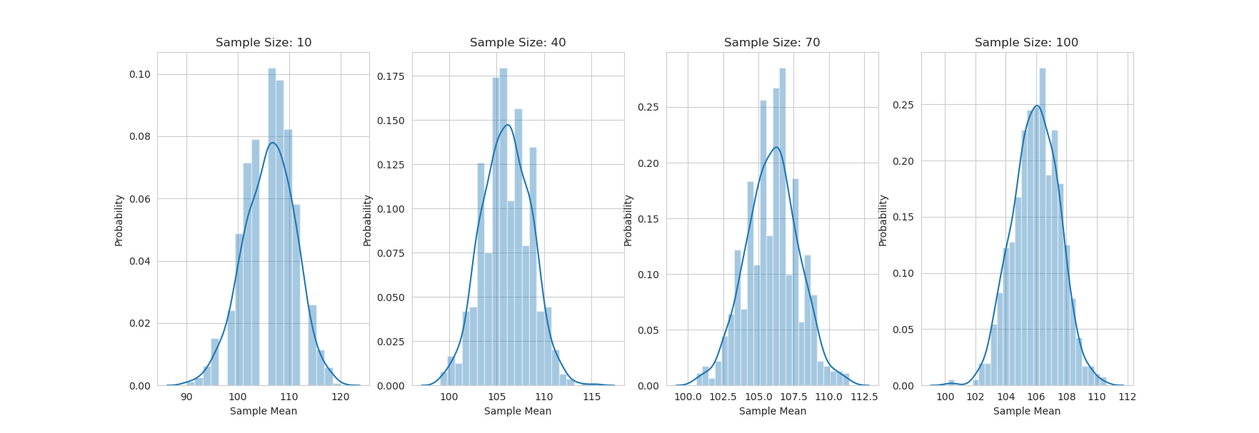
You can see that as the sample size increases, the distribution of the sample means becomes more normal (I think).
3.2. Derivation
Let's say we have a population with a mean of \(\mu\), a standard deviation of \(\sigma\) and any probability distribution. We take a random sample of size \(n\) from this population. We calculate the sample mean, and we get \(\bar{x}\). We can represent this as a random variable, \(\bar{X}\). We have to consider all the possible values of \(\bar{x}\), and their probabilities. From this, we can then calculate the distribution of \(\bar{X}\).
To now calculate the statistics for the distribution of \(\bar{X}\), we can use the following formulas
- Mean
- \(\mu_{\bar{X}} = \mu\)
- Variance
- \(\sigma_{\bar{X}}^2 = \frac{\sigma^2}{n}\) (this is also called the standard error [se])
3.3. Sample Mean
The sample mean is the most common statistic. It is the average of the sample. It is also the most common statistic to use in hypothesis testing.
We previously defined the mean and variance for sampling distributions. Now we change that up a bit. We first sum up all the random statistics \(T_O = X_0 + X_1 + \dots + X_n\). From there on, we can get the expected value and variance of this sample total:
- Expected Value
- \(E(T_O) =n \mu\)
- Variance
- \(V(T_O) = n \sigma^2\)
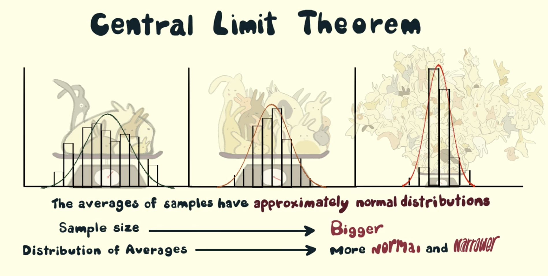
3.4. Central Limit Theorem
The central limit theorem states that the sampling distribution of the sample mean will be approximately normal, as long as the sample size is large enough.
| Population | Sample Size | Sample |
|---|---|---|
| Normal | Any | Normal |
| Unknown | Huge | Normal |
3.5. Linear Combinations
If we have a random variable \(X\), and come constants \(c\), we can define a new random variable \(Y\) as a linear combination of \(X\) and \(c\):
\[ Y = c_1 X_1 + c_2 X_2 + \dots + c_n X_n \]
Where the expected value and variance of \(Y\) are:
\[ E(Y) = c_1 E(X_1) + c_2 E(X_2) + \dots + c_n E(X_n) \]
\[ V(Y) = c_1^2 V(X_1) + c_2^2 V(X_2) + \dots + c_n^2 V(X_n) \]
For the above, we assume that the \(X_i\) are independent of each other. If they are not, we have to add the covariance terms.
\[ V(Y) = c_1^2 V(X_1) + c_2^2 V(X_2) + \dots + c_n^2 V(X_n) + 2c_1c_2Cov(X_1, X_2) + \dots + 2c_1c_nCov(X_1, X_n) + \dots + 2c_2c_nCov(X_2, X_n) \]
4. Point Estimation
With point estimation, we are trying to estimate a single value, which is the best estimate of the population parameter. We can use the sample statistics to do this.
The core idea is that if we take a random sample from a population, and calculate the sample statistics, also a random variable, we can use that to estimate the population parameter.
4.1. Properties
Generally, any estimator \(\hat{\theta}\) is just a function of the population parameter \(\theta\).
\[ \hat{\theta} = \theta + \epsilon \]
Where \(\epsilon\) is the error term. This error term is the difference between the estimator and the actual population parameter.
A way to measure the accuracy of an estimator is to use the mean squared error:
\[ MSE = \frac{1}{n} \sum_{i=1}^{n} (\hat{\theta} - \theta)^2 \]
The smaller the MSE, the better the estimator.
4.2. Estimator Bias
An estimator is unbiased only if the expected value of the estimator is equal to the population parameter. This is represented by the following formula:
\[ E(\hat{\theta}) = \theta \]
If there is any difference, that difference is the bias of the estimator.
If \(X\) is a random variable given by a binomial distribution, then \(\hat{p} = \frac{X}{n}\) is an unbiased estimator of \(p\).
We previously defined the estimate for the mean, now lets take a look at the estimate for the variance:
\[ \hat{\sigma}^2 = \frac{1}{n-1} \sum_{i=1}^{n} (x_i - \bar{x})^2 \]
This is an unbiased estimator of \(\sigma^2\).
4.3. Minimum Variance Estimators
We look at all the unbiased estimators of \(\theta\), and we choose the one with the smallest variance. This is called the minimum variance estimator.
- The less variance, the more accurate the estimator
The primary influence over the estimator, is still the original distribution.
4.4. Estimator Reporting
When we report an estimator, we have to report the standard error of the estimator. This is the standard deviation of the estimator.
- \(\hat{\theta}\) has a normal distribution
- The value of \(\theta\) lies within \(\pm 2 se\) of \(\hat{\theta}\)
- \(\hat{\theta}\) has a non-normal distribution
- The value of \(\theta\) lies within \(\pm 4 se\) of \(\hat{\theta}\)
5. Point Estimation (Methods)
5.1. Method of Moments
The method of moments is a method to estimate the parameters of a distribution. We use the sample moments to estimate the population moments. In simpler terms, we use the sample statistics to estimate the population parameters.
- What is a moment? A moment is a function of the random variable \(X\): \(E(X^k)\) (where \(k\) is the order of the moment)
The way we go about this is by using the following formula:
\[ \hat{\theta} = \frac{1}{n} \sum_{i=1}^{n} x_i^k \]
- Example
Let \(X\) be a random variable with a normal distribution with mean \(\mu\) and variance \(\sigma^2\). We take a random sample of size \(n\) from the population, and calculate the sample mean \(\bar{x}\). We want to estimate \(\mu\) using the method of moments.
Solution:
The first step to solving this problem is to find the sample mean \(\bar{x}\):
\[ \bar{x} = \frac{1}{n} \sum_{i=1}^{n} x_i \]
The next step is to find the sample variance \(s^2\):
\[ s^2 = \frac{1}{n-1} \sum_{i=1}^{n} (x_i - \bar{x})^2 \]
Now we can use the method of moments to estimate \(\mu\):
\[ \hat{\mu} = \bar{x} \]
5.2. Maximum Likelihood Estimation
Maximum likelihood estimation is a method of estimating the parameters of a statistical model, given observations. It uses calculus to find the maximum likelihood of the parameters.
First, we need a likelihood function. This is a function of the parameters, which gives the probability of the observations. The likelihood function is defined as:
\[ L(\theta) = P(X_1, X_2, \dots, X_n | \theta) \]
Where \(\theta\) is the parameter of the distribution. The likelihood function is the probability of the observations, given the parameter.
The maximum likelihood estimator is the value of the parameter that maximizes the likelihood function. This is represented by the following formula:
\[ \hat{\theta} = \underset{\theta}{\text{argmax}} L(\theta) \]
We will not be using this formula, but it is a good step to understanding. We will take our likelihood function and wrap a natural log around it. This is called the log-likelihood function. The log-likelihood function is defined as:
\[ l(\theta) = \ln L(\theta) \]
We will then take the derivative of the log-likelihood function, and set it equal to zero. This will give us the maximum likelihood estimator.
This might seem a bit pointless, but as AI students, this somewhat resembles the process of backpropagation. We take the derivative of the loss function, and set it equal to zero. This gives us the gradient of the loss function, which we can use to update the weights of the neural network. (This is a very basic explanation, but it is a good way to understand the concept)
6. Single Sample Intervals
In this section, we will look at confidence intervals for a single sample. This will combine the idea id random variables, and the idea of sampling distributions.
6.1. Confidence Intervals
This is a range between two values, which we are P% confident that the population parameter lies in. To better understand this, here is a very 'boilerplate' example:
- We choose a confidence level, \(P\).
- We get its z-score
\[ (\bar{X} - z_P \frac{\sigma}{\sqrt{n}}, \bar{X} + z_P \frac{\sigma}{\sqrt{n}}) \]
Where \(\bar{X}\) is the sample mean, and \(\sigma\) is the population standard deviation, therefore \(\frac{\sigma}{\sqrt{n}}\) is the standard error.
We can also write this as:
\[ \bar{X} \pm z_P \frac{\sigma}{\sqrt{n}} \]
So what does this tell us? It tells us that we are P% confident that the population mean lies within the interval \(\bar{X} \pm z_P \frac{\sigma}{\sqrt{n}}\).
- The more confident we want to be, the larger the confidence level \(P\). But, the larger the confidence level, the larger the interval, the lower the precision.
6.1.1. Interpretation
Since we only know \(\bar{x}, \sigma \text{ and } n\), we cannot conclude that the population mean lies within the interval \(\bar{X} \pm z_P \frac{\sigma}{\sqrt{n}}\).
Why? Because we are not using a random sample for the mean. We can only conclude that if we repeated the experiment many times, the result we obtain would occur P% of the time. In other words, if we get 100 different confidence intervals, \(P%\) of them would contain the population mean.
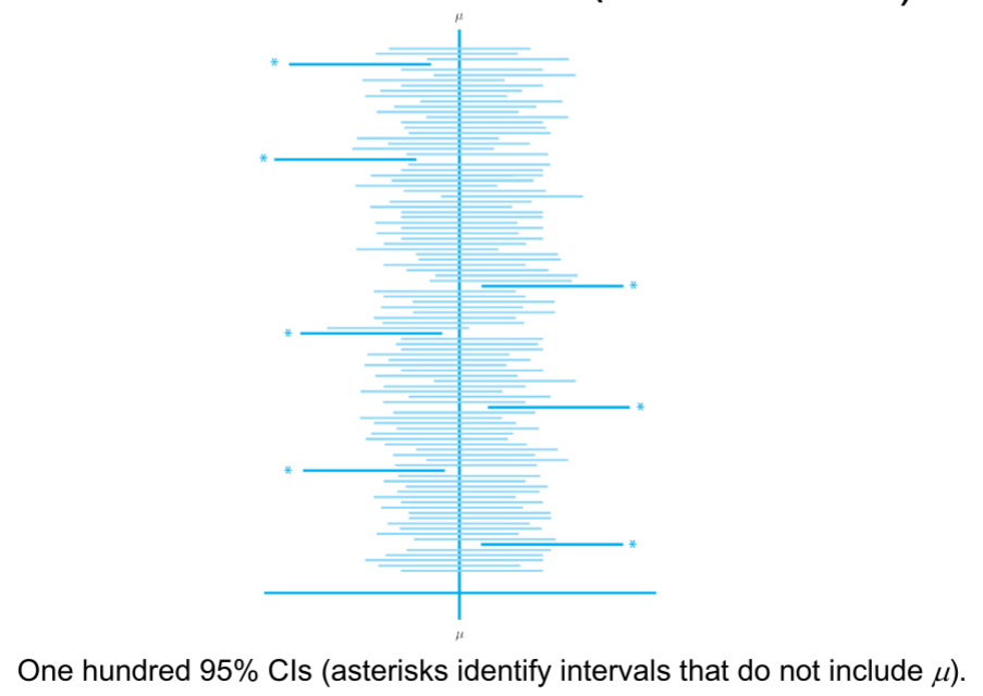
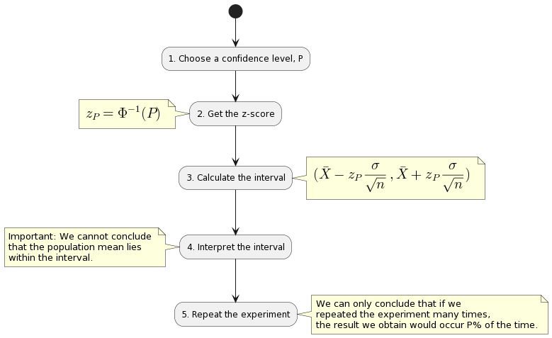
Diagram of the process of creating confidence intervals and interpreting them:
@startuml
(*) --> "1. Choose a confidence level, P"
--> "2. Get the z-score"
note left
<latex>
z_P = \Phi^{-1}(P)
</latex>
end note
--> "3. Calculate the interval"
note right
<latex>
(\bar{X} - z_P \frac{\sigma}{\sqrt{n}}, \bar{X} + z_P \frac{\sigma}{\sqrt{n}})
</latex>
end note
--> "4. Interpret the interval"
note left
Important: We cannot conclude
that the population mean lies
within the interval.
end note
--> "5. Repeat the experiment"
note right
We can only conclude that if we
repeated the experiment many times,
the result we obtain would occur P% of the time.
end note
@enduml
6.2. Confidence Levels
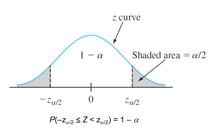
Thus far, we used a variable confidence level \(P\). But, we can also use a fixed confidence level, such as 95%. This is the same as using a confidence level of 0.95. (You must use the decimal form, not the percentage form.) Normaly, the variable which is used to represent the confidence level is \(\alpha\). So, we can write the confidence interval as:
\[ \bar{X} \pm z_{\alpha/2} \frac{\sigma}{\sqrt{n}} \]
Where \(z_{\alpha/2}\) is the z-score for the confidence level \(\alpha/2\). Why divide by 2? Because we are looking at the area under the curve on both sides of the mean. So, we are looking at the area under the curve for \(\alpha/2\) on each side of the mean.
6.3. Precision and Sample Size
First, we need to define the width of the interval as: \(2*z_P \frac{\sigma}{\sqrt{n}}\). This is the width of the interval.
- Higher the confidence level, the wider the interval.
- Higher the sample size, the narrower the interval.
- Lower the population standard deviation, the narrower the interval.
- Higher the confidence level, the higher the sample size required to achieve a given precision.
We might want to ensure, that a confidence interval has a certain width. In this case, we can use the following formula:
\[ n = (2*z_{\alpha/2} \frac{\sigma}{\text{width}})^2 \]
6.4. TODO Derivation of the Confidence Interval
If we have a random sample of size \(n\) from a population, we can construct a confidence interval for some parameter \(\theta\) using the following steps:
- Check if the conditions are met:
- The variable depends on the sample and parameter \(\theta\).
- The probability distribution of the variable is known.
7. Large Sample Confidence Intervals (Mean & Proportion)
Previously, we assumed that the population standard deviation \(\sigma\) was known and that the population distribution was normal. If we cannot assume these things, we can use the large sample confidence interval.
7.1. Large Sample Confidence Interval for the Mean
It goes back to the central limit theorem. If we take a random sample of size \(n\) from a population, we can assume that the sample mean \(\bar{X}\) is normally distributed. Therefore, we can use the following formula:
\[ Z = \frac{\bar{X} - \mu}{\frac{\sigma}{\sqrt{n}}} \]
Where \(\mu\) is the population mean, and \(\sigma\) is the population standard deviation. Thus, we can write the confidence interval as:
\[ \frac{\bar{X} - \mu}{\frac{\sigma}{\sqrt{n}}} \pm z_{\alpha/2} \]
\[ P(\frac{\bar{X} - \mu}{\frac{\sigma}{\sqrt{n}}} \pm z_{\alpha/2}) \approx 1 - \alpha \]
the last equation tells us that we are 100% - $α$% confident that the population mean lies within the interval \(\frac{\bar{X} - \mu}{\frac{\sigma}{\sqrt{n}}} \pm z_{\alpha/2}\).
What happens if we replace \(\sigma\) with \(s\) in the above equation? Since we adding a new random variable to the denominator, we get that:
- The confidence interval is wider.
But, if our sample size is large enough, the difference between \(\sigma\) and \(s\) is small, and the confidence interval is not much wider. What is large enough? If \(n \geq 40\), then the difference between \(\sigma\) and \(s\) is small enough.
7.2. Large Sample Confidence Interval for Population Proportion
Up till now we talked about being confident that the mean of a population lies within a certain interval. But, what if we want to be confident that the proportion of a population lies within a certain interval? For example, we want to be 95% confident that the proportion of people who like chocolate is between 0.4 and 0.6. We can use the following formula:
\[ P(-z_{\alpha/2} \leq \frac{\hat{p} - p}{\sqrt{\frac{p(1-p)}{n}}} \leq z_{\alpha/2}) \approx 1 - \alpha \]
Where \(\hat{p}\) is the sample proportion, \(p\) is the population proportion, and \(n\) is the sample size. Since we are talking about proportion, we are also talking about probability, and can use the binomial distribution, where \(n\) is the number of trials, and \(p\) is the probability of success. Remember that:
\begin{align} \hat{p} = \frac{X}{n} \\ E(X) = np \\ Var(X) = np(1-p) \end{align}An important rule to remember is that the sample proportion is approximately normally distributed if \(np \geq 10\) and \(n(1-p) \geq 10\).
The general formula for a confidence interval for a population proportion is:
\[ \hat{p} \pm z_{\alpha/2} \sqrt{\frac{\hat{p}(1-\hat{p})}{n}} \]
This formula can only be used if the sample size is large enough, that is if it is above 40.
7.3. One Sided
All previous confidence intervals talked about two bounds, one on the left and one on the right. But, what if we want to be confident that the population mean is greater than a certain value? For example, we want to be 95% confident that the population mean is within a certain range above the sample mean. We can use the following formula:
\[ \mu < \bar{X} + z_{\alpha} \frac{\sigma}{\sqrt{n}} \]
Where \(\mu\) is the population mean, \(\bar{X}\) is the sample mean, \(\sigma\) is the population standard deviation, and \(n\) is the sample size.
7.4. Confidence Intervals for Normal Distributions
We can assume that the population follows a normal distribution, that in only if \(n\) is large enough, (viz the central limit theorem). If we have a sample of size \(n\), then the sample mean \(\bar{X}\) is approximately normally distributed with mean \(\mu\) and standard deviation \(\frac{\sigma}{\sqrt{n}}\). We can use the following formula to calculate the confidence interval:
\[ \bar{X} \pm z_{\alpha/2} \frac{\sigma}{\sqrt{n}} \]
7.5. Confidence Interval for the t-Distribution
If we have a sample for which the mean is \(\bar{X}\) and the standard deviation is \(s\), then we can define a random variable \(T\) as:
\[ T = \frac{\bar{X} - \mu}{\frac{s}{\sqrt{n}}} \]
The distribution of \(T\) is called the Student's t-distribution. The t-distribution is similar to the normal distribution, but it has fatter tails. The t-distribution is used when the population standard deviation is unknown, and the sample size is small. The t-distribution is also used when the population distribution is not normal.
What are degrees of freedom? The degrees of freedom is the number of independent pieces of information in a sample. For example, if we have a sample of size \(n\), then the degrees of freedom is \(n-1\).
Some key properties of the t-distribution:
- It is more spread out than the normal distribution.
- The higher \(df\) is, the more similar the t-distribution is to the normal distribution.
Confidence interval for the mean using the t-distribution will then be given by this expression:
\[ \bar{X} \pm t_{\alpha, df} \frac{s}{\sqrt{n}} \]
Where \(df\) is the degrees of freedom, and \(s\) is the sample standard deviation and \(\alpha = 1 - \text{confidence level}\).
7.6. Prediction Interval for Future Values
Now we finally get to discuss future values of some variable rather than estimating what might be the mean of a population.
- We have a random sample of size \(n\). (\(X_1, X_2, \dots, X_n\))
- Now we want to know \(X_{n+1}\).
\[ E(\bar{X} - X_{n+1}) = 0 \]
\[ Var(\bar{X} - X_{n+1}) = \frac{\sigma^2}{n} + \sigma^2 = \sigma^2(1 + \frac{1}{n}) \]
Given the above, we can calculate a z-score for the confidence interval:
\[ Z = \frac{(\bar{X} - X_{n+1}) - 0}{\sigma^2 \frac{1}{\sqrt{n}}} \]
…
\[ T = \frac{(\bar{X} - X_{n+1})}{S\sqrt{1 \frac{1}{n}}} \]
From this, we can build a confidence interval for the future value of \(X_{n+1}\):
\[ \bar{x} \pm t_{\alpha, df} s \sqrt{1 + \frac{1}{n}} \]
We interpret this the same way as we did for the confidence interval for the mean. We are 95% confident that for multiple iterations, the future value of \(X_{n+1}\) will be between the two bounds.
7.7. TODO Variance and Standard Deviation Confidence Intervals
If we have a normal distribution, we might also be interested in finding the variance of the population if we do not have it. Given a sample of size \(n\), we can define a random variable as follows:
\[ \frac{(n-1)s^2}{\sigma^2} = \frac{\sum(X_i - \bar{X})^2}{\sigma^2} \]
Where \(s\) is the sample standard deviation, and \(\sigma\) is the population standard deviation. The distribution of this random variable is called the chi-squared distribution. The chi-squared distribution is used to find confidence intervals for the variance of a population.
For this distribution, we must also define the degrees of freedom. The degrees of freedom is \(n-1\).
/2023-03-11_12-13-02_.png)
Key properties of the chi-squared distribution:
- It is more spread out than the normal distribution.
- Only positive values are possible.
- The higher \(df\) is, the more similar the chi-squared distribution is to the normal distribution.
We now have to calculate the confidence interval for the variance of the population. We can do this by using the following formula:
- Lower bound: \(\frac{(n-1)s^2}{\chi^2_{\alpha/2, df}}\)
- Upper bound: \(\frac{(n-1)s^2}{\chi^2_{1-\alpha/2, df}}\)
Where \(\chi^2_{\alpha/2, df}\) is the \(\alpha/2\) percentile of the chi-squared distribution with \(df\) degrees of freedom.
We can also calculate the confidence interval for the standard deviation of the population. We can do this by using the following formula:
8. Confidence Intervals (Python)
We can make our life easier by using Python to calculate confidence intervals. We will use the following packages:
- scipy.stats
- numpy
- pandas
- matplotlib
8.1. Simple Confidence Intervals for the Mean
For ease, we will use built-in datasets from pandas, such as the iris dataset. We will use the sepal length of the iris dataset.
import pandas as pd
import numpy as np
import matplotlib.pyplot as plt
from scipy import stats

iris = pd.read_csv("https://raw.githubusercontent.com/mwaskom/seaborn-data/master/iris.csv")
sepal_length = iris["sepal_length"]
print(sepal_length.head())
0    5.1
1    4.9
2    4.7
3    4.6
4    5.0
Name: sepal_length, dtype: float64
Now we have, the data. Lets create a confidence interval for the mean of the sepal length. We will use a confidence level of 95%.
interval = stats.norm.interval(0.95, loc=np.mean(sepal_length), scale=np.std(sepal_length))
print(interval)
(4.2257725250400755, 7.460894141626592)
We can see that the confidence interval is between 4.23 and 7.46.
8.2. Confidence Interval for the Population Proportion
We will use the same dataset as before, but this time we will use the sepal width. We will use a confidence level of 95%. In the first example we do not approximate, we use the exact formula.
from statsmodels.stats.proportion import proportion_confint
# proportion where the sepal width is greater than 3.5
X = np.sum(iris["sepal_width"] > 3.5)
n = len(iris["sepal_width"])
p = X/n

interval = proportion_confint(X, n, alpha=0.05, method="normal")
print(interval)
(0.0734406885907721, 0.17989264474256125)
We can now try to approximate with the normal distribution. We will use the same confidence level of 95%.
scale = np.sqrt(p*(1-p)/n)
interval = stats.norm.interval(0.95, loc=p, scale=scale)
print(interval)
(0.07344068859077212, 0.17989264474256123)
Now lets take a look at binomial approximation for the confidence interval. We will use the same confidence level of 95%. It is important to check if the conditions are met, that is if \(np \geq 10\) and \(n(1-p) \geq 10\).
# conditions test
print("np >= 10: ", n*p >= 10)
print("n(1-p) >= 10: ", n*(1-p) >= 10)
np >= 10:  True
n(1-p) >= 10:  True
Now we can use the binomial approximation.
interval = stats.binom.interval(0.95, n, p)
print(interval)
interval = [x/n for x in interval]
print(interval)
(11.0, 27.0)
[0.07333333333333333, 0.18]
The last step is very important. We need to divide the interval by the sample size to get the proportion interval. We can see that the interval is between 0.073 and 0.18, which is a very close approximation to the normal approximation.
8.3. t Distribution Confidence Intervals
We will use the same dataset as before, but this time we will use the petal length. We will use a confidence level of 95%. In the first example we do not approximate, we use the exact formula.
from statsmodels.stats.weightstats import _tconfint_generic
# proportion where the sepal width is greater than 3.5
X = np.sum(iris["petal_length"] > 3.5)
n = len(iris["petal_length"])
p = X/n

interval = _tconfint_generic(p, np.sqrt(p*(1-p)/n), n-1, 0.05, 'two-sided')
print(interval)
(0.5555841035704419, 0.7110825630962248)
8.4. Confidence Interval for the Population Variance
We will use the same dataset as before, but this time we will use the petal width. We will use a confidence level of 95%.
s = np.std(iris["petal_width"])
var = s**2
n = len(iris["petal_width"])
alpha = 0.05
ucl = (n-1)*var/stats.chi2.ppf(alpha/2, n-1)
lcl = (n-1)*var/stats.chi2.ppf(1-alpha/2, n-1)
inteval = (lcl, ucl)
print(interval)
(0.5555841035704419, 0.7110825630962248)