Physics for Computer Science - Class Notes
Table of Contents
- 1. Electrostatic Fields
- 1.1. Electric Charge
- 1.2. Ions
- 1.3. Conductivity of Matter
- 1.4. Charging
- 1.5. Electric Polarization
- 1.6. Electric Force
- 1.7. Superposition of Forces
- 1.8. Electric Field
- 1.9. Electric Field of a Point Charge
- 1.10. Electric Field Lines
- 1.11. Uniform Electric Filed
- 1.12. Electric Flux
- 1.13. Gauss's Law
- 1.14. Electric Potential
- 1.15. Voltage
- 1.16. Electric Work
- 1.17. Electric Dipole
- 1.18. Dielectrics
- 1.19. Capacitors
- 2. Magneto-static Fields
- 2.1. Electric Current
- 2.2. Drift Velocity
- 2.3. Ohm's Law
- 2.4. Resistance
- 2.5. Resistivity
- 2.6. Electromotive Force
- 2.7. Magnetic Force
- 2.8. Magnetic Field
- 2.9. Magnetic Field Lines
- 2.10. Magnetic Flux
- 2.11. Gauss's Law of Magnetism
- 2.12. Ampere's Circuital Law
- 2.13. Magnetic Dipole
- 2.14. Hall Effect
- 3. Electromagnetism: Dynamic Fields
- 4. Waves
- 5. Electric Circuits (DC)
- 6. Electric Circuits (AC)
- 7. Matter
- 8. Energy Bands
- 9. Semiconductors (Equilibrium)
- 10. Semiconductors (Non-Equilibrium)
- 11. PN Junctions
- 12. Transistors
- 13. Quantum Mechanics
- 14. Final Project
- 15. References
- 16. Mind Map
New search feature! Make use of the amazing fuzzy search algorithm. Just type in the search box and it will find the closest match in the page. Hit Enter to jump to the next match. Lmk if it doesn't work for you.
There are 4 fundamental forces in nature: Gravity, Electromagnetism, Weak Nuclear Force and Strong Nuclear Force. Electromagnetic forces rely on particles which have a charge.
1. Electrostatic Fields
1.1. Electric Charge
Charge, is something as fundamental as mass. It is what determines how intense electromagnetic forces are. Here are some fundamental laws which govern charge:
- Charge is conserved. If you have a positive charge, you can't have a negative charge. If you have a negative charge, you can't have a positive charge.
- Charge is quantized. Charge is measured in units of elementary charge, which is \(e = 1.602176634 \times 10^{-19} C\). This means that you can't have a charge of \(1.5e\).
- Charge is additive. If you have two charges, you can add them together to get the total charge. For example, if you have a charge of \(+1e\) and a charge of \(-1e\), you can add them together to get a total charge of \(0e\).
- Opposite charges attract, and like charges will repel.
1.2. Ions
An Ion is just a charged particle. It is a particle which has a charge. For example, a proton is an ion with a charge of \(+1e\). A neutron is an ion with a charge of \(0e\). An electron is an ion with a charge of \(-1e\).
- What determines if an Ion is positive or negative?
- It is determined by the number of protons and electrons. If the number of protons is greater than the number of electrons, then the Ion is positive. If the number of electrons is greater than the number of protons, then the Ion is negative. If the number of protons is equal to the number of electrons, then the Ion is neutral.
1.3. Conductivity of Matter
There are three main types:
- Insulators
- This type of matter does not conduct electricity. For example, glass is an insulator.
- Semiconductors
- This type of matter is a bit of an in-between. It can conduct electricity, but not very well. For example, silicon is a semiconductor.
- Conductors
- This type of matter conducts electricity very well. For example, copper is a conductor.
1.4. Charging
We can charge on object in three ways: Friction, Induction and Conduction.
- Friction
- This is when you rub two objects together. For example, if you rub a balloon on your hair, you will get a static charge on the balloon. Here the electrons are transferred from your hair to the balloon through friction.
- Induction
- This is when you bring a charged object near another object.
- Conduction
- Electrons get transferred from one object to another, through direct contact.
1.5. Electric Polarization
If you have a neutrally charged object and you subject it to an electric field, it will become polarized. Meaning that the electrons will move to one side of the object, and the protons will move to the other side of the object.
- Why does this happen?
- Because bodies charges have a tendency to align themselves with the electric field.
1.6. Electric Force
This is a force which is exerted between two charged objects. It is given by the equation, also knows as Coulomb's Law:
\[ F = k \frac{q_1 q_2}{r^2} \]
Where \(k\) is the Coulomb constant, \(q_1\) and \(q_2\) are the charges of the two objects, and \(r\) is the distance between the two objects. The simplest definition of \(k\) is:
\[ k = \frac{1}{4 \pi \epsilon_0} \]
Where \(\epsilon_0\) is the permittivity of free space. The permittivity of vacuum is a constant which is equal to \(8.8541878128 \times 10^{-12} F/m\).
We can generally approximate \(k\) as:
\[ k = 9 \times 10^9 N \cdot m^2/C^2 \]
The electric force abides by the third law of Newtonian mechanics. This means that if object \(A\) exerts a force on object \(B\), then object \(B\) will exert a force on object \(A\) which is equal in magnitude, but opposite in direction.
1.7. Superposition of Forces
Give two charges, \(q_1\) and \(q_2\) and a third charge \(q_3\), the net force on \(q_3\) is given by the vector sum of the forces exerted by \(q_1\) and \(q_2\).
Vector sum: 15.2
1.8. Electric Field
How do charges exert forces on other charges? They do so through the electric field. The electric field is a vector field which is defined as:
\[ \vec{E} = \frac{\vec{F}}{q} \]
Where \(F\) is the force exerted on the charge, and \(q\) is the charge. The electric field is a vector field, which means that it has a direction and a magnitude. The direction of the electric field is the direction of the force. The magnitude of the electric field is the magnitude of the force divided by the charge.
Useful video on electric field: https://www.youtube.com/watch?v=bHIhgxav9LY
We can re-arrange this equation to get the force exerted on a specific point:
\[ \vec{F} = q \vec{E} \]
For this to be possible, we need to know the electric field at that point. We can find the electric field at a point by many means. This is also only valid for point charges.
Some other key properties of the electric field:
- The electric field is a vector field. This means that it has a direction and a magnitude.
- Inside a conductor, the electric field is zero.
1.9. Electric Field of a Point Charge
The electric field of a point charge is given by:
\[ \vec{E} = \frac{k q}{r^2} \hat{r} \]
Where \(k\) is the Coulomb constant, \(q\) is the charge of the point charge, and \(r\) is the distance between the point charge and the test charge. The electric field is a vector field, which means that it has a direction and a magnitude.
1.10. Electric Field Lines
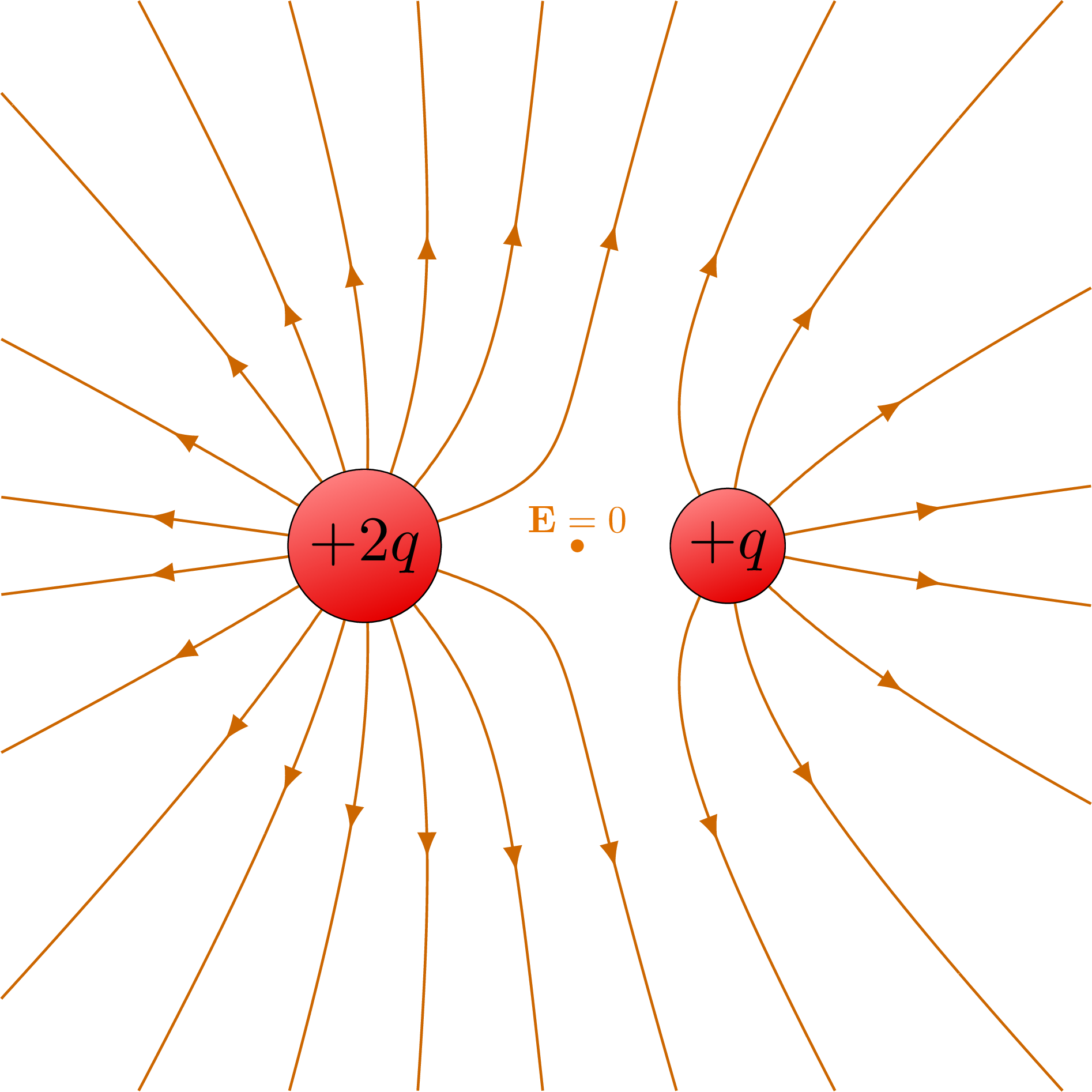
One of the most important properties of the electric field is that it is symmetrical. The spacing of the lines is proportional to the magnitude of the electric field. The closer the lines are together, the stronger the electric field. The further apart the lines are, the weaker the electric field. The direction of the lines is the direction of the electric field.
- The electric field lines are a visual representation of the electric field. They are not a physical object.
1.11. Uniform Electric Filed
A uniform electric field is an electric field which is constant in all directions. The electric field lines are parallel to each other, and are equidistant from each other. The electric field lines are also perpendicular to the surface of the object.
Although not electric, gravity can be thought of as a uniform field, at least near the surface of the earth. It only goes down.
1.12. Electric Flux
The electric flux is the amount of electric field passing through a surface. It is given by the equation:
\[ \Phi = \int_S \vec{E} \cdot d\vec{A} \]
The flux will primarily depend on two factors: the angle relative to the surface and which side of the surface we are measuring.
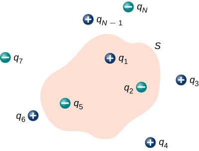
1.13. Gauss's Law
It equates flux, to the charge enclosed by the surface. It is given by the equation:
\[ \Phi = \frac{Q}{\epsilon_0} \]
Where \(\Phi\) is the electric flux, \(Q\) is the charge enclosed by the surface, and \(\epsilon_0\) is the permittivity of free space. The permittivity of vacuum is a constant which is equal to \(8.8541878128 \times 10^{-12} F/m\).
It is valid for anything. When we talk about an enclosed surface, it does not have to be a physical surface.
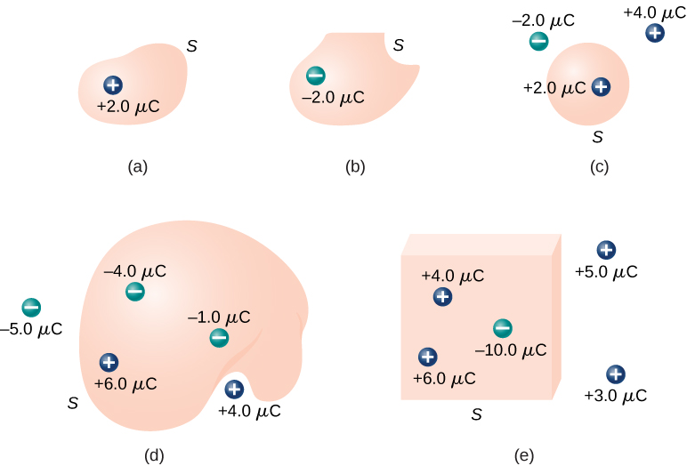
- \(\Phi = \frac{2.0 \mu C}{\epsilon_0} = 2.3 \times 10^5 N \cdot m^2/C\)
- \(\Phi = -\frac{2.0 \mu C}{\epsilon_0} = -2.3 \times 10^5 N \cdot m^2/C\)
- \(\Phi = \frac{2.0 \mu C}{\epsilon_0} = 2.3 \times 10^5 N \cdot m^2/C\)
- \(\Phi = \frac{4.0 \mu C + 6.0 \mu C - 1.0 \mu C}{\epsilon_0} = 1.1 \times 10^5 N \cdot m^2/C\)
- \(\Phi = \frac{4.0 \mu C + 6.0 \mu C - 10.0 \mu C}{\epsilon_0} = 0\)
1.13.1. Gauss's Law for Conductors
In a conductor, the electric field is zero. Any excess charge will only be at the surface. This means that
1.14. Electric Potential
First we have to understand the concept of potential energy. Potential energy is the energy that an object has due to its position (or configuration). It is given by the equation:
\[ U = mgh \]
This is gravitational potential energy.
Electric potential energy is the amount of work that needs to be done when moving a unit charge against an electric field. It is given by the equation:
\[ V(\vec{r}) = \frac{1}{4\pi\epsilon_0} \frac{q_1}{\vec{r} - \vec{r}^\prime} \]
Where \(V(\vec{r})\) is the electric potential energy, \(\epsilon_0\) is the permittivity of free space, \(q_1\) is the charge, \(\vec{r}\) is the position of the charge, and \(\vec{r}^\prime\) is the position of the point where we are measuring the electric potential energy.
The entire system is also governed by:
\[ \vec{E} = -\nabla V (\vec{r}) \]
Where \(\vec{E}\) is the electric field, \(\vec{r}\) is the position vector, and \(V\) is the electric potential.
The scalar function for the electric potential is called the electric potential function. It is given by the equation:
\[ U = q_1 \cdot V(\vec{r}) \]
Where \(U\) is the electric potential energy, \(q_0\) is the charge, and \(V\) is the electric potential.
Some key points about the electric potential:
- If a force does positive work, then the potential energy decreases
- The slightest difference in potential energy. We must have some sort of reference point where \(U = 0\), this is called the ground.
1.15. Voltage
Voltage is the difference in electric potential energy between two points. It is given by the equation:
\[ V = V_2 - V_1 \]
Where \(V\) is the voltage, \(V_1\) is the electric potential energy at point 1, and \(V_2\) is the electric potential energy at point 2.
1.16. Electric Work
Here we are talking about a force acting on a moving particle. The work done by the force is given by the equation:
\[ W = \int \vec{F} \cdot d\vec{r} \]
Where \(W\) is the work done, \(\vec{F}\) is the force, and \(\vec{r}\) is the position vector. This is what is called a 15.3.
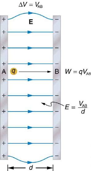
If we are in an uniform electric field, the work done by the electric field is given by the equation:
\[ W_{a\to b} = Fd = q_0 Ed \]
Where \(W_{a\to b}\) is the work done by the electric field, \(F\) is the force, \(q_0\) is the charge, \(E\) is the electric field, and \(d\) is the distance.
1.17. Electric Dipole
An electric dipole is a system of two equal and opposite charges separated by a distance \(d\). The electric dipole moment is given by the equation:
\[ \vec{p} = q_0 \vec{d} \]
Where \(\vec{p}\) is the electric dipole moment, \(q_0\) is the charge, and \(\vec{d}\) is the distance between the two charges. What is a moment? It is a measure of how much an electric field will rotate a dipole. The electric dipole moment is a vector quantity.
If we take a dipole, and pop it into an electric field, it will rotate to align itself. The torque is given by the equation:
\[ \vec{\tau} = \vec{p} \times \vec{E} \]
Where \(\vec{\tau}\) is the torque, \(\vec{p}\) is the electric dipole moment, and \(\vec{E}\) is the electric field. This is just an extra.
What is important, is the potential energy of a dipole. The potential energy of a dipole is given by the equation:
\[ U = -\vec{p} \cdot \vec{E} \]
Where \(U\) is the potential energy, \(\vec{p}\) is the electric dipole moment, and \(\vec{E}\) is the electric field.
1.18. Dielectrics
This is an insulator, that gets polarized when an electric field is applied. The polarization is the separation of charge.
We talked a lot about permittivity and dielectric constant. The permittivity of a dielectric is given by the equation:
\[ \epsilon = \epsilon_0 \epsilon_r \]
Where \(\epsilon\) is the permittivity, \(\epsilon_0\) is the permittivity of free space, and \(\epsilon_r\) is the relative permittivity.
You can find a table of relative permittivity here: 15.4.
1.19. Capacitors
A capacitor is like a battery, but it stores energy in the form of electric charge. It consists of two conductors separated by an insulator.
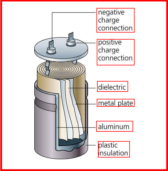
How do we charge a capacitor? We can charge it by connecting it to a battery. The battery will supply a constant current to the capacitor. The capacitor will charge up until the voltage across the capacitor is equal to the voltage of the battery. The current will then stop flowing.
The capacitance of a capacitor is given by the equation:
\[ C = \frac{Q}{V} \]
Where \(C\) is the capacitance, \(Q\) is the charge, and \(V\) is the voltage. This is given in the units of Farads.
Some factors which affect the capacitance:
- The area of the plates
- The distance between the plates
- The permittivity of the dielectric
The capacitance of a parallel plate capacitor is given by the equation:
\[ C = \frac{\epsilon_0 A}{d} \]
Where \(C\) is the capacitance, \(\epsilon_0\) is the permittivity of free space, \(A\) is the area of the plates, and \(d\) is the distance between the plates.
2. Magneto-static Fields
2.1. Electric Current
This is pretty much the same type of current as we can observe in water. It is the flow of charge through space. That is why, we can define it as a function of time and space \(Q(\vec{r})\), or better yet, represent it as a derivative the previous function:
\[ I = \frac{dQ}{dt} \]
Where \(\vec{I}\) is the current, \(Q\) is the charge, and \(t\) is time. Alternatively, we can define it as:
\[ I = nqv_d A \]
Where \(I\) is the current, \(n\) is the number of particles per unit volume, \(q\) is the charge of a single particle, \(v_d\) is the drift velocity, and \(A\) is the cross-sectional area which we are focusing on. Current is not a vector, but it is a scalar quantity. It is a measure in amperes (A).
2.1.1. Vector Current Density
What is this? It is the current per unit volume. It is given by the equation:
\[ \vec{J} = nq\vec{v_d} \]
Where \(\vec{J}\) is the vector current density, \(n\) is the number of particles per unit volume, \(q\) is the charge of a single particle, and \(\vec{v_d}\) is the drift velocity. The magnitude is given by the equation:
\[ \vert \vec{J} \vert = I / A \]
Where \(\vert \vec{J} \vert\) is the vector current density, \(I\) is the current, and \(A\) is the cross-sectional area.
The key difference here is that the current is a scalar quantity, and the vector current density is a vector quantity.
2.2. Drift Velocity
We have already mentioned this a few times. To better understand what this is, imagine a lot of bouncy-balls thrown into a tube. If we look at a certain part of the tube, we can see that the bouncy-balls are moving in all directions, but if we zoom out and look at the tube as a whole, we can see that the bouncy-balls are moving in one direction. This is the drift velocity.
Now replace the tube with a wire, and the bouncy-balls with charges. The drift velocity is the average velocity of the charges in a wire. There will be a certain electric field which goes through the wire, the negative charges will feel a force opposite to the direction of the electric field, and they will move in the direction opposite of the electric field.
- Negative charges move against the electric field
- Positive charges move with the electric field
2.3. Ohm's Law
Here we focus on the law in vector form. This means that we are going to focus on the vector current density, and not the current. The law is given by the equation:
\[ \vec{J} = \sigma \vec{E} \]
Where \(\vec{J}\) is the vector current density, \(\sigma\) is the conductivity, and \(\vec{E}\) is the electric field. We can also replace \(\sigma\) with \(\rho\) but have to adjust a bit, since \(\rho\) is the resistivity. The equation then becomes:
\[ \vec{J} = \frac{1}{\rho} \vec{E} \]
2.4. Resistance
Resistance is the opposition to the flow of current. It is given by the equation:
\[ R = \rho L / A \]
Where \(R\) is the resistance, \(\rho\) is the resistivity, \(L\) is the length of the wire, and \(A\) is the cross-sectional area of the wire. The units of resistance are ohms (\(\Omega\)).
2.5. Resistivity
Resistivity is the resistance per unit length. It is given by the equation:
\[ \rho = \frac{R}{L} \]
Where \(\rho\) is the resistivity, \(R\) is the resistance, and \(L\) is the length of the wire. The units of resistivity are ohm-meters (\(\Omega m\)).
Important not to confuse the two.
2.6. Electromotive Force
Another day another force. This is the force which causes the current to flow. It is given by the equation:
\[ \Epsilon = V_{ab} \]
Where \(\Epsilon\) is the electromotive force, and \(V_{ab}\) is the voltage between two points. The units of electromotive force are volts (\(V\)).
2.7. Magnetic Force
Now things might get a bit tricky. This is a force which occurs due to the motion of charges. It is given by the equation:
\[ \vec{F} = \frac{\mu_0}{4\pi} \frac{q\vec{v}\times\vec{B}}{r^2} \]
Where \(\vec{F}\) is the magnetic force, \(\mu_0\) is the permeability of free space, \(q\) is the charge, \(\vec{v}\) is the velocity, \(\vec{B}\) is the magnetic field, and \(r\) is the distance between the charge and the magnetic field. The units of magnetic force are newtons (\(N\)).
Thats a hell of a lot of variables. Lets break it down a bit.
- \(\mu_0\) is the permeability of free space
- \(q\) is the charge
- \(\vec{v}\) is the velocity
- \(\vec{B}\) is the magnetic field
- \(r\) is the distance between the charge and the magnetic field
The key conceptual thing here is the cross product of two vectors. This is a vector perpendicular to both vectors. This is the direction of the magnetic force. How can we better understand this? We use the right hand rule. If we have two vectors, we can put our right hand in the direction of the first vector, we then curl our fingers in the direction of the second vector, and our thumb will point in the direction of the cross product. This is the direction of the magnetic force.
2.8. Magnetic Field
When a charge moves, it creates a magnetic field. This is given by the equation:
\[ \vec{F} = q\vec{v}\times\vec{B} \]
Where \(\vec{F}\) is the magnetic force, \(q\) is the charge, \(\vec{v}\) is the velocity, and \(\vec{B}\) is the magnetic field. The units of magnetic field are tesla (\(T\)).
Some key concepts related to the magnetic field:
- The magnetic field is a vector quantity
- It is always perpendicular to the velocity of the charge
2.9. Magnetic Field Lines
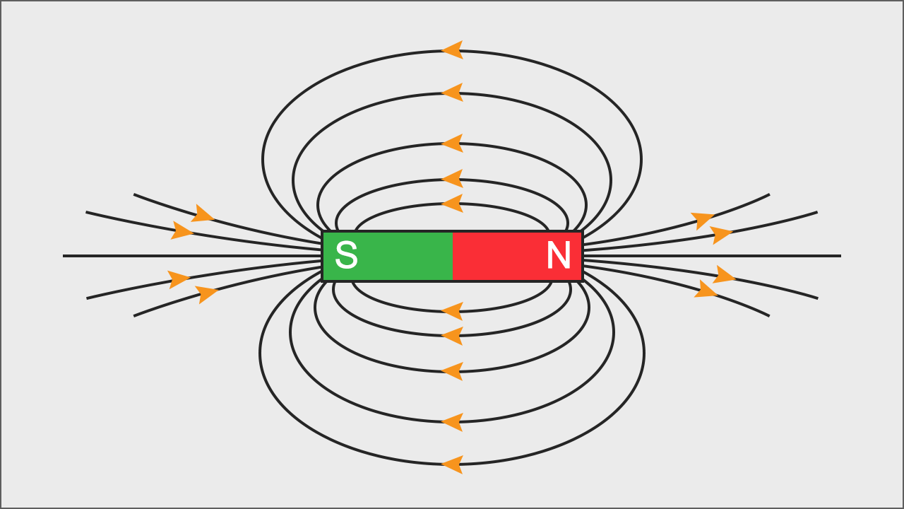
The magnetic field lines are the lines which show the direction of the magnetic field. They are perpendicular to the velocity of the charge. The magnetic field lines are closed loops.
They share some traits with the electric field lines:
- They spacing is proportional to the magnitude of the field
- They never intersect
2.10. Magnetic Flux
Similar to the electric flux, this is the amount of magnetic field passing through a surface. It is given by the equation:
\[ \Phi = \int_S \vec{B}\cdot d\vec{A} \]
Where \(\Phi\) is the magnetic flux, \(\vec{B}\) is the magnetic field, and \(d\vec{A}\) is the differential area. The units of magnetic flux are webers (\(Wb\)).
2.11. Gauss's Law of Magnetism
When you take a magnet, split it in half, each half will still have two poles. This is because the magnetic field is continuous. This is the law of magnetism. It is given by the equation:
\[ \oint_C \vec{B}\cdot d\vec{l} = 0 \]
Where \(\oint_C\) is the integral around a closed loop, \(\vec{B}\) is the magnetic field, and \(d\vec{l}\) is the differential length. The units of Gauss's Law of Magnetism are tesla-meters (\(Tm\)).
2.12. Ampere's Circuital Law
2.13. Magnetic Dipole
2.14. Hall Effect
3. Electromagnetism: Dynamic Fields
3.1. Motional Electromotive Force
If we have a conductive object moving through a magnetic field, it will create an electromotive force. This is given by the equation:
\[ \epsilon = \cint \vec{v} \times \vec{B} \cdot d\vec{l} \]
Where \(\epsilon\) is the motional electromotive force, \(\vec{v}\) is the velocity, \(\vec{B}\) is the magnetic field, and \(d\vec{l}\) is the length of the conductive object. The units of motional electromotive force are volts (\(V\)).
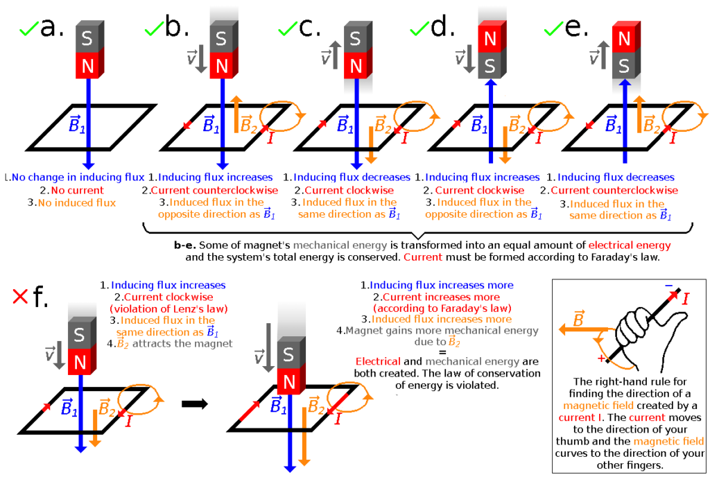
3.2. Faraday's Law of Induction
In this law, we learn that a change in the magnetic flux, will create an electromotive force. You can also think of the change of flux as the second derivative of the magnetic field. This is given by the equation:
\[ \epsilon = -\frac{d\Phi}{dt} \]
Where \(\epsilon\) is the motional electromotive force, \(\Phi\) is the magnetic flux, and \(t\) is time. The units of Faraday's Law of Induction are volts per second (\(V/s\)).
- If the flux is changing, only then will there be an electromotive force
- A change in flux, does not only depend on the magnetic field, but also the area of the surface.
The direction of an electromotive force is given by the right hand rule. Since the law of induction has a minus sign in front of it, the direction of the electromotive force is opposite to the direction which will be indicated by the right hand rule, unless the flux is changing.
3.3. Lenz's Law
The induced emf or current in a circuit opposes the change in magnetic flux. This law describes the natural tendency of a circuit to resist any change in the magnetic flux.
3.4. Alternators
An alternator is device which converts mechanical rotational energy into electrical energy. It is a type of generator which makes use of the Faraday's Law of Induction. It is given by the equation:
\[ \epsilon = -N\frac{d\Phi}{dt} = -\frac{d}{dt} (BA \cos{\omega t}) = \omega B A \sin{\omega t} \]
Where \(\epsilon\) is the motional electromotive force, \(N\) is the number of turns, \(\Phi\) is the magnetic flux, \(t\) is time, \(\omega\) is the angular frequency, \(B\) is the magnetic field, and \(A\) is the area. The units of alternators are volts (\(V\)).
3.5. Self-Inductance
First, we need to redefine the emf as the change in current, because if we have a circuit, which is in a steady state, the emf will be zero, unless there is a change in current. This is given by the equation:
\[ \epsilon = -L\frac{dI}{dt} \]
Where \(\epsilon\) is the motional electromotive force, \(L\) is the self-inductance, \(I\) is the current, and \(t\) is time. The units of self-inductance are henrys (\(H\)).
3.6. Inductors
We can see self-inductance in circuits with these components:

To calculate the self-inductance, we need to know the number of turns, the area of the coil, and the magnetic field. This is given by the equation:
\[ L = \frac{\muN^2 A}{2 \pi R} \]
In a circuit we represent the component with a coil-like symbol. Why would we want to use such a component? Well, we can use it to store energy. This is because the emf is proportional to the change in current, and the change in current is proportional to the change in voltage. This means that if we have a circuit with a battery, and an inductor, the current will increase, and the voltage will decrease. This is because the battery is trying to increase the current, but the inductor is trying to decrease the current. This is called an inductive reactance.
3.7. Mutual Inductance
If we have two coils, and we change the current in one coil, the other coil will also change its current. This is because the magnetic field is changing, and the magnetic field is changing because the current is changing.
For these kinds of problems, it is important to remember that any change in the magnetic field will create an electromotive force.
3.8. Eddy Currents
Eddy currents, are currents which are created by a changing magnetic field. Although this might not be good for fine technology, as it can interfere, here are some applications of eddy currents:
- Metal Detectors - detect eddy currents in metal
- Heating - eddy currents create heat
- Magnetic Breaking
4. Waves
4.0.1. Displacement Current
If the electric field changes, so will the magnetic field. This is because the magnetic field is proportional to the electric field.
We take amperes circuital law, and include the magnetic field:
\[ \oint_C \vec{B}\cdot d\vec{l} = \mu_0 (i_c + i_D)_\text{enc} \]
where:
\[ i_D = \epsilon_0 \frac{d\Phi_E}{dt} \]
Where \(\Phi_E\) is the electric flux, and \(t\) is time. The units of displacement current are amperes (\(A\)).
4.0.2. Maxwell's Equations
Finally, the good stuff. Maxwell's equations are the equations which describe the relationship between the electric and magnetic fields. They are given by the equations:
\begin{align} \oint \vec{E} \cdot d\vec{A} &= \frac{Q_{enc}}{\epsilon_0} \\ \oint \vec{B} \cdot d\vec{A} &= 0 \\ \oint \vec{B} \cdot d\vec{A} &= \mu_0 (i_c + i_D)_\text{enc} \\ \oint \vec{E} \cdot d\vec{A} &= - \frac{d\Phi_B}{dt} \end{align}This is a compilation of:
- Gauss's Law for Electric Fields
- Gauss's Law for Magnetic Fields
- Extended Ampere's Law
- Faraday's Law of Induction
They will often be expressed in differential form:
\begin{align} \nabla \cdot \vec{E} &= \frac{\rho}{\epsilon_0} \\ \nabla \cdot \vec{B} &= 0 \\ \nabla \times \vec{E} &= -\frac{\partial \vec{B}}{\partial t} \\ \nabla \times \vec{B} &= \mu_0 (\vec{J} + \vec{D})_\text{enc} \end{align}4.0.3. Electromagnetic Waves
The key relationship here, is modeled by these equations:
\begin{align} \oint \vec{B} \cdot d\vec{l} &= \epsilon_0 \mu_0 \frac{d}{dt}\int\vec{E} \cdot d\vec{A} \\ \oint \vec{E} \cdot d\vec{l} &= -\frac{d}{dt}\int\vec{B} \cdot d\vec{A} \end{align}One of the most important properties, is \(\vec{k}\). This is the wave vector, and it is given by:
\[ \vec{k} \tilda \vec{E} \times \vec{B} \]
Also, all waves in a vacuum travel at the speed of light, which is given by:
\[ c=\frac{1}{\sqrt{\mu_{0} \varepsilon_{0}}}=2.99792458 \times 10^{8} \mathrm{m} / \mathrm{s} \]
4.0.4. Monochromatic Plane Waves
We first need to understand a wave in 1D:
\[ y(x,t) = A \sin(kx - \omega t) \]
Where \(A\) is the amplitude, \(k\) is the wave number, and \(\omega\) is the angular frequency. The units of the wave number are radians per meter (\(rad/m\)). The units of the angular frequency are radians per second (\(rad/s\)).
Now, we can extend this to 3D:
\[ E(\vec{r},t) = \vec{E}_\text{max} \cos(k\ctod\vec{r} - \omega t) \]
Thats pretty awful looking, now we make it even worse by splitting it into two components, each wave being for the electric and magnetic fields:
\begin{align} \vec{E}(x,t) &= \hat{j} \vec{E}_\text{max} \cos(k\vec{r} - \omega t) \\ \vec{B}(x,t) &= \hat{k} \vec{B}_\text{max} \cos(k\vec{r} - \omega t) \end{align}Where \(\hat{j}\) and \(\hat{k}\) are unit vectors in the \(x\) and \(y\) directions respectively. The units of the magnetic field are tesla (\(T\)).
4.0.5. Electromagnetic Spectrum
4.0.6. Poyntig Vector
4.0.7. Electromagnetic Waves on Boundaries
4.0.8. Standing Waves
5. Electric Circuits (DC)
5.1. Circuits
First, we need to define some terms:
- Terminal
- The point where a component is connected to a circuit
- Connection
- A wire, which has no resistance, and connects two terminals.
- Node or Junction
- A point where two or more connections meet.
- Loop
- A closed path in a circuit.
- Branch
- A path in a circuit, which is not a loop and has no nodes.
- Mesh
- A closed path in a circuit, which has no branches or no internal loops.
5.2. Passive Components
These are components which absorb energy, they are the following:
5.2.1. Resistors
Resistors are components which have a resistance. The resistance \(R\) is given by:
\[ R = \rho \frac{l}{A} \]
Where \(\rho\) is the resistivity, \(l\) is the length, and \(A\) is the cross-sectional area. The units of resistance are ohms (\(\Omega\)).
We can combine resistors, either in series or in parallel. In series, the total resistance is the sum of the individual resistances. In parallel, the total resistance is the sum of the reciprocals of the individual resistances.
How can you calculate the resistance of a resistor, based on the bands? The first two bands are the first two digits of the resistance, the third band is the multiplier, and the fourth band is the tolerance.
You can use this tool to calculate the resistance of a resistor, based on the bands.
5.2.2. Capacitors
This component accumulates charge. The capacitance \(C\) is given by:
\[ C = \frac{Q}{V} \]
Where \(Q\) is the charge, and \(V\) is the voltage. The units of capacitance are farads (\(F\)).
As for the order, it is reversed from resistors. Capacitance in series is given by the sum of the reciprocal of the individual capacitances. Capacitance in parallel is given by the sum of the individual capacitances.
5.2.3. Inductors
An inductor is a component which stores energy in the form of a magnetic field. The inductance \(L\) is given by:
\[ L = \frac{\Phi}{I} \]
Where \(\Phi\) is the flux, and \(I\) is the current. The units of inductance are henrys (\(H\)).
Parallel inductors are given by the sum of the reciprocal of the individual inductances. Series inductors are given by the sum of the individual inductances.
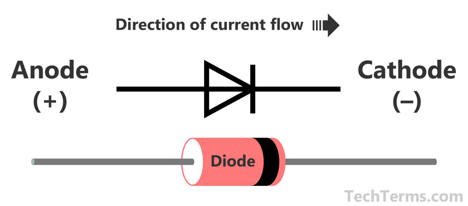
5.2.4. Diodes
A diode is a component which allows current to flow in one direction, and blocks it in the other.
There is a special type of diode, the light emitting diode (LED). This is a diode which emits light when current flows through it.
5.3. Active Components
These are components which generate energy, they are the sources of energy in a circuit. They can supply current or voltage.
5.3.1. Current Supplying Components
| Current | Voltage |
|---|---|
| Fixed | Variable |
Graphically, the current supplying components are the following:
/2023-02-23_14-33-46_screenshot.png)
5.3.2. Voltage Supplying Components
| Current | Voltage |
|---|---|
| Variable | Fixed |
Graphically, the voltage supplying components are the following:
/2023-02-23_14-53-41_screenshot.png)
5.4. Electrical Measurements
To measure almost everything in a circuit, you need a multimeter. This is a device which can measure voltage, current, and resistance.
Usually looks something like this:
/2023-02-23_14-55-44_6_000_Count_True_RMS_High_Performance_Waterproof_IP67_Digital_Multim_%E2%80%94_Triplett_Test_Equipment_Tools.jpg)
5.5. Kirchoff's Laws
This law tells us that the sum of currents in a node, or the sum of voltages in a loop, is always zero.
\[ \sum_j I_j = 0 \]
Why? Since a node, has not property which would allow it to cumulate charge, the current must be zero.
This also means, that the current leaving a node, must be equal to the sum of the currents entering the node.
We can apply this to a circuit, but constructing equations for each of the nodes. We can then solve these equations to find the currents in the circuit.
As for loops, we know that the sum of all the voltages in a loop is zero. This means that the voltage drop across each component in the loop must be equal to the voltage drop across the loop.
5.6. Transient and Steady-State
A transient state is a state where the circuit is changing with respect to time. Whereas a steady-state is a state where the circuit that has constant or period magnitudes.
- For a steady state, the current and voltage are constant.
- For a transient state, the current and voltage are changing.
5.7. RC Circuits
An RC circuit is a type of circuit which contains a resistor and a capacitor connected in series or parallel to each other. The resistor controls the amount of current running through the circuit and the capacitor acts as a storage device for electric charge.
These two components work to create a transient state and steady state within the RC circuit, which means that the current and voltage in the circuit will initially change over time before reaching a steady, constant rate.
The RC circuit is used in many applications, such as in the power supply of a computer, in the circuitry of a radio, and in the circuitry of a television.
5.8. Electric Power
In classical mechanics, power is defined as the rate of doing work. In electromagnetism, power is defined as the rate of energy transfer. The power \(P\) is given by:
\[ P = \frac{dW}{dt} = \frac{VdQ}{dt} = VI \]
Probably the nicest equation in this course. The units of power are watts (\(W\)).
5.9. TODO Mesh Analysis
Mesh analysis is a method of solving a circuit, by constructing equations for each of the meshes in the circuit. We can then solve these equations to find the currents in the circuit.
- Identify all the meshes in the circuit.
- Apply the Kirchoff's Voltage Law to each of the meshes.
- Solve the equations to find the currents in the circuit.
5.10. Circuit Theorems
5.10.1. Superposition Theorem
Just as any other application of the superposition theorem.
The superposition theorem states that the current in a circuit is the sum of the currents in the circuit, when each of the sources are turned on one at a time.
5.10.2. Thevenin's Theorem
Given any circuit with multiple voltages and resistances, we can replace the circuit with a single voltage source and a single resistance. This helps us decrease complexity in our circuits.
Why? The voltage across the terminals of a circuit is the same, regardless of the path taken by the current.
5.11. Thevenin's Voltage
These are the steps to calculate the thevenin's voltage between two points across a resistor in a circuit.
6. Electric Circuits (AC)
These are circuits, that run on alternating current. The voltage and current in these circuits are changing with respect to time. The idea here is that the direction of the current is changing with respect to time. It is given by:
\[ V(t) = V_p \sin(\omega t) \]
Where \(V_p\) is the peak voltage, and \(\omega\) is the angular frequency. The units of angular frequency are radians per second (\(rad/s\)). You might ask, what is peak voltage? It is the maximum voltage in the circuit.
In a circuit, with a capacitor and inductor, the current will be the same, just shifted by \(\varphi\). This is given by:
\[ I(t) = I_p \sin(\omega t + \varphi) \]
Where \(I_p\) is the peak current, and \(\varphi\) is the phase difference between the voltage and current. The units of phase difference are radians (\(rad\)).
So where can we see AC current? The most common place is in the powerlines leading to our house.
6.1. Complex Numbers
It is important to note, that we can use complex numbers only with linear circuits.
6.2. Impedance
The impedance \(Z\) of a circuit is given by the following. This is also called the generalized ohm's law.
\[ Z = \frac{V}{I} \]
We can then take this general formula, and apply it to resistors, inductors and capacitors. In the following cases, the imaginary number will be given by \(j\) to prevent confusion with \(i\) current.
6.2.1. Resistor
The impedance of a resistor is given by:
\[ v_r = i_r R \]
\[ i_r = I_R e^{j\omega t} \]
If we substitute this into the general formula, we get:
\[ v_r = R I_R e^{j\omega t} \]
6.2.2. Inductor
The impedance of an inductor is given by:
\[ v_L = L \frac{di_L}{dt} \]
\[ i_L = I_L e^{j\omega t} \]
If we substitute this into the general formula, we get:
\[ v_L = L I_L j\omega e^{j\omega t} \]
6.2.3. Capacitor
The impedance of a capacitor is given by:
\[ i_C = C \frac{dv_C}{dt} \]
\[ v_C = V_C e^{j\omega t} \]
If we substitute this into the general formula, we get:
\[ i_C = C V_C j\omega e^{j\omega t} \]
6.2.4. Respective Impedances
This is probably the most important part:
| Impedance | Formula |
|---|---|
| Resistor | \(R\) |
| Inductor | \(j\omega L\) |
| Capacitor | \(\frac{1}{j\omega C}\) |
6.3. AC Power
The power \(P\) in an AC circuit is given by:
\[ P = V(t) I(t) = V_p \sin{\omega t} I_p \sin{\omega t + \varphi} \]
We can also compute the average power, which is the power that is being delivered to the circuit. This is given by:
\[ P_{avg} = \frac{1}{T} \int_{0}^{T} P(t) dt \]
Where \(T\) is the period of the circuit.
Now, we bring out the complex numbers. The power in an AC circuit is given by:
\[ P = V I^* \]
Where \(I^*\) is the complex conjugate of the current. The complex conjugate can be found here. We can re-write this as:
\[ S = \vert V \vert ^2 Z = \frac{|V|^2}{Z^*} \]
Where \(S\) is the complex power, and \(Z^*\) is the complex conjugate of the impedance. We can also re-write this as:
\[ P = |S| \cos(\varphi) \]
Where \(\theta\) is the phase difference between the voltage and current.
6.4. Reactive Power
What is reactive power? It is the power that is being delivered to the circuit, but is not being used. This is given by:
\[ Q = VI \sin{\varphi} \]
6.5. Resonance Frequency
The resonance frequency is the frequency at which the impedance of the circuit is zero. This is given by:
\[ \omega_r = \frac{1}{\sqrt{LC}} \]
When resonance occurs, the current and voltage are in phase. This is given by:
- \(\phi = \tan^-1{0} = 0\)
- \(I_p = \frac{V_p}{R}\)
- \(Z = R\)
We might also want to see the quality of the resonance. This is given by:
\[ Q = \frac{\omega_r}{\delta \omega} \]
Where \(\delta \omega\) is the bandwidth of the circuit.
7. Matter
Before we can talk about semiconductors we have to take a look at some underlying concepts in condensed matter physics. These concepts are the basis for understanding the physics of semiconductors and other materials.
7.1. Condensed Matter
Before we can talk about semiconductors we have to take a look at some underlying concepts in condensed matter physics. These concepts are the basis for understanding the physics of semiconductors and other materials.
Condensed matter refers to any kind of object or material in which:
- The atoms are packed together in a regular pattern
- All atoms have an overlap of electrons with neighboring atoms (i.e. they are not free to move around)
We can classify materials into two categories:
- Crystalline materials
- Amorphous materials
7.2. Crystalline Materials
We will only focus on crystalline materials for now. This is a bit of a rough concept, here is an analogy to help you understand it:
Imagine you are a kid and you are playing with a bunch of legos. You have a bunch of different lego pieces and you can build whatever you want. You can build a house, a car, a robot, whatever you want. This is an amorphous material.
Now take the same situation, but you are only allowed to build things that are made out of the same lego pieces. This is a crystalline material.
We commonly use the term latices to describe the arrangement of atoms in a crystalline material. The most common lattices are:
| Lattice | Image |
|---|---|
| Cubic | 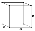 |
| Body Centered | 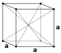 |
| Face Centered | 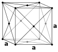 |
7.3. Bonding in Crystalline Materials
In physics/chemistry a bond is just like any other, it is a force that holds two atoms together. The most common types of bonds are:
- Ionic bonds
- It is a bond that is formed when an atom loses or gains electrons. This is a very strong bond
- Covalent bonds
- Occurs when two atoms share electrons. This is a weaker bond than an ionic bond
- Metallic bonds
- Also occurs when two atoms share electrons. The main difference is that the electrons are free to move around. This is the weakest bond
Why is this important? Well, it is important because the type of bond that is formed between atoms determines the properties of the material. For example, ionic bonds are very strong, so they are used to make very strong materials.
7.4. Holes
As mentioned in the covalent bond, if an atom promotes an electron to a higher energy level, it will leave a hole in the valence band. This hole is called a hole. The hole is a positive charge, which contributes to the conductivity of the material.
8. Energy Bands
The next step before we can talk about semiconductors is to talk about energy bands. Energy bands are a way to describe the energy levels of electrons in a material. We create diagrams to demonstrate these energy bands for each atom. This diagram is called an energy-level diagram, here is an example for Hydrogen:
| n | Energy (eV) |
|---|---|
| 1 | -13.6 |
| 2 | -3.4 |
| 3 | -1.5 |
| 4 | -0.85 |
| 5 | -0.54 |
Between each level \(n\) there is a gap of energy. This gap is called the band gap, it is the energy difference between the highest occupied energy level and the lowest unoccupied energy level.
- Highest occupied energy level
- The highest energy level that has electrons in it
- Lowest unoccupied energy level
- The lowest energy level that does not have electrons in it
The gaps matter, because they determine the properties of the material. Primarily they determine the conductivity of the material. The higher the band gap, the less conductive the material is. The lower the band gap, the more conductive the material is.
Why is this? Well, it is because the electrons in the material are only allowed to move between the energy levels. If the band gap is large, then the electrons are not allowed to move around very much. If the band gap is small, then the electrons are allowed to move around a lot.
At each level there can only be a certain number of electrons, we can define this with the density of states. The density of states is the number of states per unit energy. This is given by:
\[ n(E) = \frac{1}{\Delta E} \]
Where \(\Delta E\) is the energy difference between each level. This is also known as the Fermi-Dirac distribution.
8.1. Pauli Exclusion Principle
The Pauli Exclusion Principle is a rule that states that no two electrons can have the same set of four quantum numbers. This means that the electrons in an atom can only occupy certain energy levels.
8.2. Valance and Conduction Bands
- Conduction band
- The first band at which there are no electrons
- Valance band
- The last band at which there are electrons
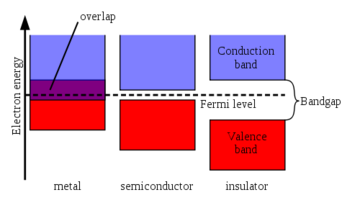
The above figure shows three different energy-bands structures for metal, semiconductor, and insulator. The band gap is the energy difference between the valance band and the conduction band. The higher the band gap, the more insulating the material is. The lower the band gap, the more conductive the material is.
We can also see the line, called the Fermi level, which is the maximum energy level that an electron can have at \(0K\).
9. Semiconductors (Equilibrium)
At last, we can talk about semiconductors. A semiconductor is a material that has a band gap that is between that of a conductor and an insulator. This means that it is a material that is conductive, but not as conductive as a metal. The range in which the band gap can be is \(0.5 \Leftrightarrow 2.5\) eV.
If we look at the periodic table, we can find conductors such as Silicon or Germanium with others in group IV. 15.1
9.1. Doping
Just like in sports, doping is the act of adding a substance to a material to improve its performance. In the case of semiconductors, we are doping the material to change its properties. There are two types of doping:
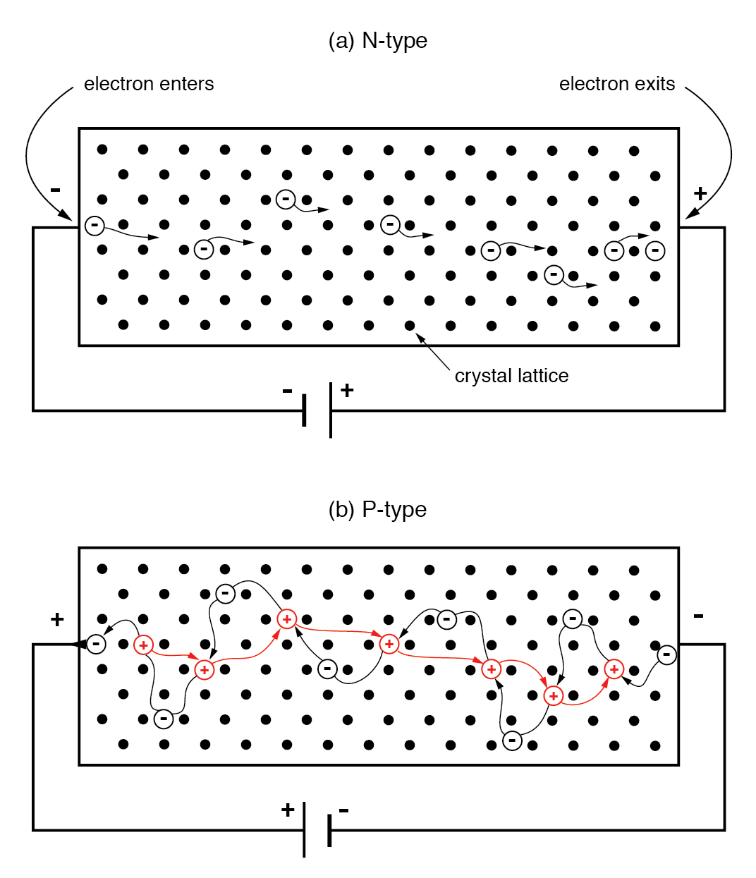
- N-type doping
- Adding an impurity that has 5 valence electrons (such as Phosphorus) to a material.
- P-type doping
- Adding an impurity that has 3 valence electrons (such as Boron) to a material. Like this, we create holes in the valance band.
/2023-03-09_16-43-48_.png)
9.2. Intrinsic vs Extrinsic Conductivity
So if we dope a material, we either create excess electrons or holes. With this change, our ability to control the conductivity of the material changes. We can control the conductivity of the material with temperature.
So what dose intrinsic and extrinsic mean? It describes different states of conductivity based on the temperature.
9.3. Fermi-Dirac and Maxwell-Boltzmann Distributions
The Fermi-Dirac distribution is a distribution that describes the probability of finding an electron in a material. It is given by:
\[ f(E) = \frac{1}{e^{\frac{E - E_F}{kT}} + 1} \]
Where \(E_F\) is the Fermi level, \(k\) is the Boltzmann constant, and \(T\) is the temperature. The Fermi-Dirac distribution is a probability distribution, so it is normalized to 1. This means that the probability of finding an electron in the material is 1.
- \(k = 1.38 \times 10^{-23} J/K\)
/2023-03-09_17-09-49_.jpeg)
We can approximate the Fermi-Dirac distribution with the Maxwell-Boltzmann distribution. The Maxwell-Boltzmann distribution is given by:
\[ f(E) = \frac{1}{e^{\frac{E}{kT}} + 1} \]
Where \(E\) is the energy of the electron, \(k\) is the Boltzmann constant, and \(T\) is the temperature. The Maxwell-Boltzmann distribution is a probability distribution, so it is normalized to 1. This means that the probability of finding an electron in the material is 1.
9.4. Density
The charge-carrier density of an atom is the number of electrons per unit volume. This is given by:
\[ n_0 = \frac{1}{V} \int_{E_F}^{\infty} n(E) dE = \frac{1}{V} \int_{E_F}^{\infty} g_n(E) f(E) dE \]
10. Semiconductors (Non-Equilibrium)
10.1. Drift Velocity
If we have some charge, without the presence of an electric field, it will move in an erratic manner. They move at a thermal speed \(v_T\). With statistics, we can say:
\[ \frac{1}{2} m v_T^2 = \frac{3}{2} kT \]
Where \(m\) is the mass of the electron, \(k\) is the Boltzmann constant, and \(T\) is the temperature. Typically, we can say that \(v_T = 10^7 cm/s\). If we now apply an electric field, the charge carriers will move in the direction of the electric field. This is called the drift velocity \(v_D\). The drift velocity is given by:
\[ v_D = \frac{q}{m} \tau \]
Where \(q\) is the charge of the electron, \(m\) is the mass of the electron, and \(\tau\) is the relaxation time, which can also be seen in this equation:
\[ m * \frac{dv}{dt} = qE - \frac{m}{\tau} v \]
Finally, we can say that the net velocity of the charge carriers is given by:
\[ v(t) = v_D exp(-t/\tau) \]
As time goes to ∞ the charge carriers will reach equilibrium. This is called the diffusion length \(L_D\).
10.2. Mobility
Now that we have the drift velocity, we can calculate the mobility. The mobility is given by:
\[ \mu = \frac{\vert \vec{v_D} \vert}{\vert \vec{E} \vert} \]
Where \(\vec{v_D}\) is the drift velocity and \(\vec{E}\) is the electric field. Mobility tells us the strength of drift velocity given a certain electric field.
Some important notes about mobility:
- Depends on the impurity of the material
- It holds that:
- $n$-type materials have a higher mobility than $p$-type materials
- \(m_n \neq m_p \land \tau_n \neq \tau_p\) (the mobility of electrons and holes are different)
With some fancy math we get to:
\[ \frac{1}{\mu} = \frac{1}{\mu_\text{vib}} + \frac{1}{\mu_\text{imp}} = AT^{3\over2} + BT^{-3\over2} \]
Where \(A\) and \(B\) are constants, \(T\) is the temperature, and \(\mu_\text{vib}\) and \(\mu_\text{imp}\) are the mobility due to vibration and impurity, respectively. We can see that the mobility is inversely proportional to the temperature to the power of \(3/2\).
/2023-03-19_13-44-59_screenshot.png)
10.3. Drift Current
The drift current is the current that is caused by the drift velocity of the charge carriers. The drift current is given by the following equations, respectively to each type of carrier (n/p):
\[ j_n = \frac{I_n}{A} = en\mu_n E \]
\[ j_p = \frac{I_p}{A} = ep\mu_p E \]
Where \(I_n\) and \(I_p\) are the current of the electrons and holes, respectively, \(A\) is the area of the cross-section of the material, \(e\) is the charge of the electron, \(n\) and \(p\) are the electron and hole densities, respectively, \(\mu_n\) and \(\mu_p\) are the mobility of the electrons and holes, respectively, and \(E\) is the electric field. The drift current is the current that is caused by the drift velocity of the charge carriers. We can also get the net drift current by adding the two currents together:
\[ J_{\text{total}} = e(n\mu_n + p\mu_p) E = \sigma E \]
Where \(\sigma\) is the conductivity of the material. The conductivity is the current per unit voltage. We can also say that the drift current is the current that is caused by the drift velocity of the charge carriers.
10.4. Electric Conductivity in Semiconductors
First we need to understand what is really meant by "intrinsic".
Being or relating to a semiconductor in which the concentration of charge carriers is characteristic of the material itself instead of the content of any impurities it contains
In simpler terms: intrinsic semiconductors are semiconductors that have no impurities. Intrinsic semiconductors have a very high resistivity, which means that they have a very low conductivity. This is because the charge carriers are not free to move around. They are bound to the atoms.
Now, we need to define the electric mass action law: \(n_i^2 \prop \exp(-E_g/kT)\). With this, we can now rewrite \(\sigma\) (the conductivity) as:
\[ \sigma(T) = \sigma_0 \exp(-E_g/2kT) \]
Where \(\sigma_0\) is the conductivity at \(T=0\), \(E_g\) is the band gap energy, \(k\) is the Boltzmann constant, and \(T\) is the temperature. We can see that the conductivity is inversely proportional to the temperature to the power of \(2\). This is because the charge carriers are more free to move around at higher temperatures.
For better interpretation, we can rewrite the equation as:
\[ \ln(\sigma) = -(\frac{E_g}{2k}) \frac{1}{T} + \ln(\sigma_0) \]
/2023-03-19_14-02-24_screenshot.png)
10.5. Photoconductivity
/2023-03-19_14-03-51_.png)
Above is a Feynman diagram in which we can see the electrons emit photons when they are excited. This is called the photoelectric effect. We can now relate this to semiconductors:
If we expose a semiconductor to an EM wave, the electrons will be excited and have make the material more conductive. They do this by jumping from the valance band to the conduction band.
10.6. Hall Effect in Semiconductors
[SYS]: You are Richard Faynman
[ME]: What is the Hall effect in semiconductors?
[AI]: The Hall effect is a fundamental phenomenon in condensed matter physics that occurs when an electric current flows through a semiconductor or other material in the presence of a magnetic field perpendicular to the direction of the current. The interaction between the moving charges in the current and the magnetic field causes a measurable voltage perpendicular to both the current and the magnetic field, which is known as the Hall voltage. This effect is used in a range of electronic devices, such as sensors, transducers, and magnetic field measurement instruments. The Hall coefficient, which is defined as the ratio of the Hall voltage to the product of the current and magnetic field, is a key parameter used in the characterization of semiconductors and other materials with electronic properties.
We previously looked at the Hall effect in metals. In semiconductors, the Hall effect is caused by the presence of the electric field. The magnetic field will cause the charge carriers to move in a direction perpendicular to the electric field. This will cause a voltage to appear across the material. This voltage is called the Hall voltage.
\[ V_H = E_y W \]
For each type of semi conductor, we can define a Hall coefficient:
- For n-type semiconductors
- \(R_H = \frac{-1}{en}\)
- For p-type semiconductors
- \(R_H = \frac{1}{ep}\)
Where \(W\) is the width of the material, \(E_y\) is the electric field in the y-direction, \(e\) is the charge of the electron, \(n\) is the electron density, and \(p\) is the hole density.
With these values, we can also get the mobility of the charge carriers:
\[ \mu = \sigma R_H = \frac{V_B L}{V_0 B_z W} \]
Where \(V_B\) is the voltage across the material, \(L\) is the length of the material, \(V_0\) is the voltage across the material, \(B_z\) is the magnetic field in the z-direction, and \(W\) is the width of the material.
10.7. Inhomogeneous Semiconductors
This is a kind of semiconductor that has a non-uniform distribution of charge carriers. This is caused by the presence of impurities. Possible causes:
- Doping
- Inhomogeneous light
10.8. Diffusion Current
If we have a bunch of charge carriers concentrated in one part of the material, they will diffuse to the other parts of the material. This is called diffusion. The diffusion current is the current that is caused by the diffusion of the charge carriers. It can be modeled mathematically:
\[ j = -D \nabla n = -D \frac{\partial c}{\partial x} \]
Where \(j\) is the diffusion current, \(D\) is the diffusion coefficient, \(\nabla\) is the gradient operator, \(n\) is the charge carrier density, and \(c\) is the concentration of the charge carriers.
Again, we can define this with respect to each type of charge carrier predominant in a semiconductor:
- n-type
- \(J_n \vert_{text{diff}} = eD_n \frac{\partial n}{\partial x}\)
- p-type
- \(J_p \vert_{text{diff}} = - eD_p \frac{\partial p}{\partial x}\)
10.9. Generation and Recombination of Charge Carriers
We can generate an electron-hole pair if we direct a photon to an electron. When the photon hits the electron, the electron jumps into a higher energy state, it also leaves a hole behind in the valance band.
If we go the other way around, we can recombine an electron-hole pair. This happens when the electron and the hole combine to form a neutral atom. This is called radiative recombination. This recombination also releases a photon.
11. PN Junctions
If we put two semiconductors together, we get a PN junction. Each of the semiconductors must respectively have the n-type and p-type doping. The resulting junction is called a diode.
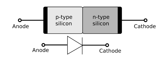
Based on the voltage provided, the region between the two semiconductors, will have a different potential. This is also called the depletion region. The depletion region is where the charge carriers are not free to move around. This region allows for current to flow in one direction only. A diode like this will often be used in a circuit to prevent current from flowing in the wrong direction, for example, if changing AC to DC.

The depletion region, is created when some electrons from the n-type switch sides with the holes from the n-type. Inherently, this switch, creates an electric field which sustains the depletion region. This is called the built-in electric field.
11.1. In Equilibrium
For a diode to reach a state of equilibrium, we need to have the following conditions:
- The drift current is equal to the diffusion current for each type of charge carrier
What is diffusion current? It is the current that is caused by the diffusion of the charge carriers.
11.2. Polarized Junctions
If we put a pn-junction into an EM field, we will see different outcomes for the depletion and neutral region.
- Forward Bias
- If we apply voltage to the p side of the junction, the depletion region deceases in potential. Current can flow in this direction.
- Reverse Bias
- If we negative apply voltage to the n side of the junction, the depletion region increases in potential. Current cannot flow in this direction.
We can define the width of that region by:
\[ W=\sqrt{\frac{2 \varepsilon (V_{b i}-V)}{e} \frac{N_{A}+N_{D}}{N_{A} N_{D}}} \]
Where \(\varepsilon\) is the permittivity of the material, \(V_{b i}\) is the built-in voltage, \(V\) is the applied voltage, \(e\) is the charge of the electron, \(N_{A}\) is the concentration of acceptors, and \(N_{D}\) is the concentration of donors.
11.3. Characteristic I-V Curve of the Diode
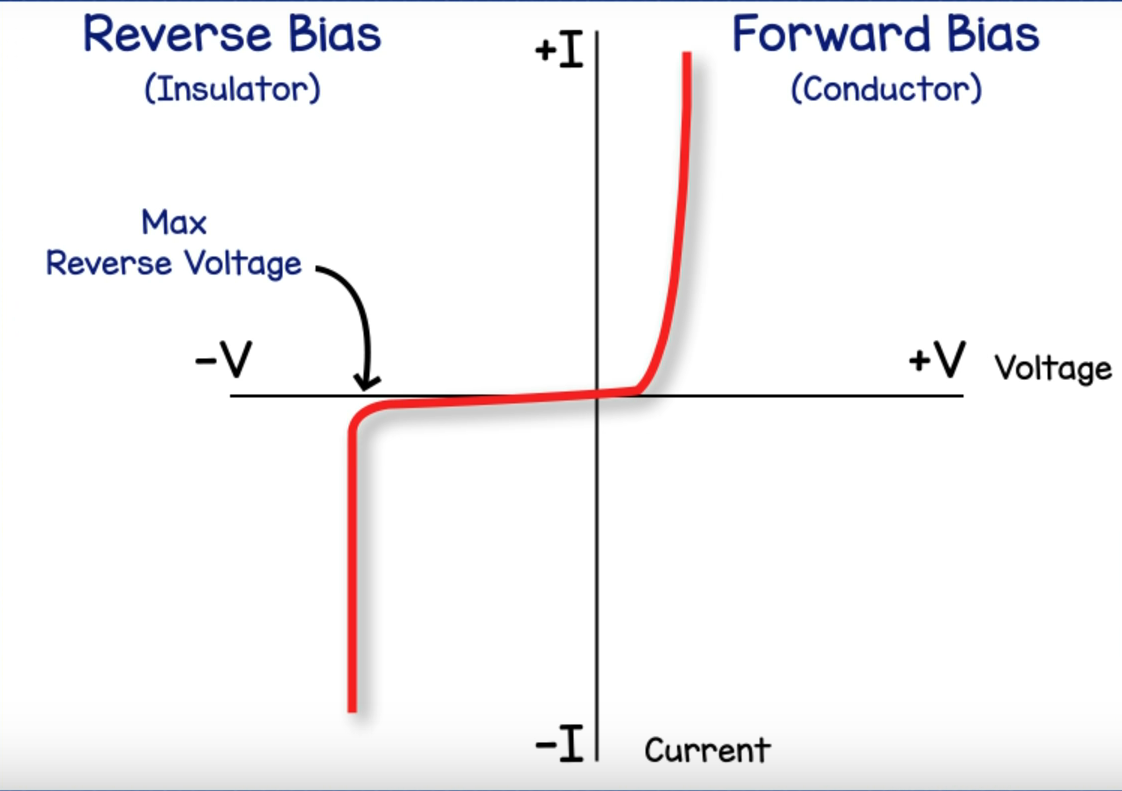
This curve gives us the behavioral property of the device. It tells us how the diode will behave in the circuit when we apply a voltage to it.
11.4. LEDs and Lasers
An LED is a special kind of diode, that emits light when current is applied to it. The light is emitted when the electrons jump from the valance band to the conduction band. This is called the photoelectric effect. The light is emitted in the form of photons. The color of the light is determined by the band gap energy of the semiconductor. The higher the band gap energy, the more energy is required to excite the electrons. This means that the light emitted will have a higher frequency and thus a higher energy. This is why the color of the light is red (for example).
- Anode
- Longer leg = Positive
- Cathode
- Shorter leg = Negative
11.5. Optoelectronic Devices
What is this? It is a device that uses light to control the electrical properties of a semiconductor. This is done by using the photoelectric effect.
11.6. Diodes in Circuits
- Guess at how the diode will pass (forward or reverse) bias
- Replace diode with a voltage source (usually .7V)
- Solve for current
- If it makes sense, you are done, if not, go back to step 1 and switch your bias.
12. Transistors
12.1. Bipolar Junction Transistors
12.1.1. Basic Functioning
12.1.2. Polarization
12.1.3. Modeling
12.1.4. Circuit Analysis with Transistors
12.1.5. Digital Circuits
12.2. MOSFETs
12.2.1. Work Function
12.2.2. MOS
12.2.3. MOSFET
12.2.4. Qualitative Functioning
12.2.5. Polarization
12.2.6. Modeling
12.2.7. Circuit Analysis with MOSFETs
12.2.8. CMOS
12.2.9. Logic Gates with CMOS
12.3. Comparison of Bipolar and MOSFETs
13. Quantum Mechanics
13.1. Laws of Quantum Physics
13.2. Superconducting Circuits
14. Final Project
14.1. Project Proposal
14.2. Project Report
15. References
15.1. Periodic Table

15.2. Vector Sum
A vector sum is just the addition of two vectors. For example, if you have two vectors, \(\vec{a}\) and \(\vec{b}\), then the vector sum of \(\vec{a}\) and \(\vec{b}\) is given by:
\[ \vec{a} + \vec{b} = \begin{bmatrix} a_x \\ a_y \end{bmatrix} + \begin{bmatrix} b_x \\ b_y \end{bmatrix} = \begin{bmatrix} a_x + b_x \\ a_y + b_y \end{bmatrix} \]
15.3. Line Integral
A definite integral gives use the area under the curve. This is done by taking very small slices of the curve and adding them together. A line integral is the same thing, but instead of taking slices of the curve, we take slices of the line and then multiply the slides by the vector filed.
15.4. Relative Permittivity Table
Equation for permittivity of a dielectric:
\[ \epsilon = \epsilon_0 \epsilon_r \]
\[ \epsilon_0 = 8.854187817 \times 10^{-12} \text{ F/m} \]
| Material | Relative Permittivity |
|---|---|
| Air | 1.0059 |
| Water | 80.000 |
| Glass | 4.0000 |
| Diamond | 9.0000 |
| Silicon | 11.000 |
| Teflon | 2.1000 |
| Mylar | 2.2000 |
| Copper | 1.0000 |
| Gold | 1.0000 |
15.5. Complex Numbers
The most common format of a complex number is: \(x + iy\) where \(x\) is the real part and \(y\) is the imaginary part. The imaginary part is denoted by \(i\), but \(i\) iteself is not the imaginary part.
\[ i = \sqrt{-1} \]
The imaginary part is denoted by \(j\) in some cases.
- Modulus of a complex number
- \(\vert z \vert = \sqrt{x^2 + y^2}\)
- Conjugate of a complex number
- \(\bar{z} = x - iy\)
- Euler representation
- \(z = r e^{i\theta}\)
- Polar representation
- \(z = r e^{i\theta} = r(\cos\theta + i\sin\theta)\)
- Addition
- \(z_1 + z_2 = (x_1 + x_2) + i(y_1 + y_2)\)
16. Mind Map
