Fundamentals of Probability and Statistics - Problem Set 4
These notes should cover continuous random variables and the probability distributions associated.
Probability Density Functions (\(pdf\))
- Discrete Random Variables \(rv\)
- This is a variables which can take on a some values from a finite set. If this variable can take on the entire interval of numbers, it is not discrete.
The pdf, should give us the probability for the variable it is taking in as input. The pdf (probability density function) for some random variable \(X\) is defined by the area between two points of interest:
\[ P(a \le X \le b) = \int_a^b f(x) dx \]
The rules for defining a pdf are:
- \(\forall x [f(x) > 0]\)
- \(\int_{-\infty}^{\infty} f(x) dx = 1\)
For a this kind of distribution, the probability for a singular point will be 0, this is because the interval on the range of 0 will always be 0. This is in fact very useful, because it allows for this to be true:
\[ P(a \le X \le b) \equiv P(a < X < B) \]
Where it does not matter if we use \(\le \lor <\) or \(\ge \lor >\).
Cumulative Distribution Functions (\(cdf\))
This functions, gives the area of the \(pdf\), for the range defined by \(-\infty,x\) where x is a parameter which the \(cdf\) takes on.
\[ F(x) = P(X \le x) = \int_{-\infty}^{\infty} f(y) dy \]
The notation is similar to calculus, where the anti-derivative of a functions is defined by \(F\). This can be useful to get a better intuition of what is going on. Some useful rules for computing probabilities with these distributions are as follows:
- \(P(X > a) = 1 - F(a)\)
- \(P(a \le X \le b) = F(b) - F(a)\)
Expected Values
The expected values, which is also the mean, is given by the following formula:
\[ \mu_x = E(X) = \int_{-\infty}^{\infty} x * f(x) dx \]
Where the \(f(x)\) is the probability distribution function. If we are interested in computing the mean for the \(x\) value which is given by another functions \(h(x)\), we simply replace the \(x\) in the above formula with \(h(x)\).
Variance
For a discrete random variable \(X\), its variances is defined as follows:
\[ \sigma_x^2 = V(X) = \int_{-\infty}^{\infty} (x - \mu)^2 * f(x) dx = E[(X - \mu)^2] \]
And the standard deviation is of course $σx = \sqrt{V(x)}. We can also calculate the variance just by using the expected values:
\[ V(X) = E(X^2) - E(X)^2 \]
In this case, \(E(X^2)\) is given by \(\int_{-\infty}^{\infty} x^2 f(x) dx\).
The Normal Distribution
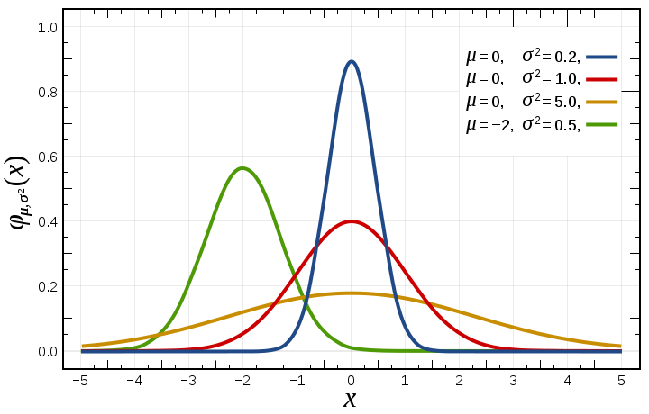
This distribution can be seen in many parts of the worlds, most notably people thinks its what the distribution of IQ looks like, over the past few years, it has been show to be turning more skewed (IQ has flaws). The normal distribution is defined by two parameters: \(\mu\) and \(\sigma\). The function which defines the distribution is messy and complicated:
\[ f(x; \mu, \sigma) = \frac{1}{\sqrt{2\pi}\sigma} e^{-(x-\mu)^2 \over 2\sigma^2} \]
Being defined over \(-\infty < x < \infty\). The way you might see it denoted is by \(X ~ N(\mu, \sigma^2)\). Quite intuitively, the expected value is given by \(\mu\) and the variance by \(\sigma^2\). If we want to compute the probability on some interval, we would have to integrate the above function, this would be slow and painful. For this reason, to get the cumulative function, we use z-scores. If we want to compute the value for some percentile in the distribution, we can look at the z-score table in reverse.
Nonstandard Normal Distribution
We can change the values of the distribution by adjusting the \(\mu\) and \(\sigma\).
Usage to Approximate the Binomial Distribution
We can get the approximation of a binomial distribution, by knowing its mean and variation, using this we can estimate a normal distribution, that is, as long as the original binomial distribution is not too skewed. Since \(\mu = np\) and \(\sigma = \sqrt{npq}\).
\[ P(X \le x) = B(x,n,p) = \phi(\frac{x+5 - np}{\sqrt{npq}}) \]