Fundamentals of Probability and Statistics - Midterm 1
Table of Contents
- 1. Fundamental Elements of Statistics
- 2. Graphically Descriptive Statistics
- 3. Descriptive Statistics
- 3.1. Percentiles
- 3.2. Quartiles
- 3.3. Mean
- 3.4. Median
- 3.5. Trimmed Means
- 3.6. Skew
- 3.7. Distribution Shape
- 3.8. Frequency
- 3.9. Sample Variance
- 3.10. Sample Standard Deviation
- 3.11. Population Variance
- 3.12. Population Standard Deviation
- 3.13. The Range
- 3.14. Outliers
- 3.15. Statistical Robustness
- 3.16. Chebychev's Theorem
- 3.17. Empirical Rules
- 3.18. Z Score
- 3.19. Correlation
- 3.20. Sample Proportions
- 3.21. Hypothesis Testing
- 4. Probability
- 4.1. Sample Space
- 4.2. Events
- 4.3. Axioms of Probability
- 4.4. Properties of Probability
- 4.5. Operations with Probability
- 4.6. Systematic Approach to Solving Probabilities
- 4.7. Uniform Probabilities
- 4.8. Product Rule for Ordered Pairs
- 4.9. Permutations
- 4.10. Combinations
- 4.11. Conditional Probability
- 4.12. Bayes' Theorem
- 4.13. Independence
- 5. Appendix 1
- Date
- 2nd November
1. Fundamental Elements of Statistics
1.1. Data Matrix
A collection of data categorized by each class of data. For a data matrix, each row (an observation) can be called a case, observational unit or experimental unit.
1.2. Types of Variables
All variables can be categorized into two categories: numerical and categorical.
- Numerical
- This type of data can either be continuous or discrete. It can take a wide range of numerical values.
- Categorical
- If some data can be put into different (usually finite) groups, it will be categorical.
- Ordinal
- Ordinal variables are those that are categorical, but have a numerical order.
1.3. Explanatory and Response Variables
When we are trying to find a relationship between two variables, we need to identify which is the explanatory and which is the response variable. We usually assume that the explanatory affects the response variable.
\[ \text{explanatory} \to \text{ might affect } \to \text{response} \]
1.4. Types of Data Collection
In statistics, there are two main ways we might collect data. We use observational studies or experiments.
1.4.1. Observational studies
When conducting a study of this kind, there is no interference with data generation i.e. there are no treatments or controls. Most common way collecting this data is with surveys.
- Observational Data
- Data which is generated without any treatment being applied
- Causal Conclusions
- Cannot be made without experimentation. We can however note that there might be an association.
1.4.2. Experiment
In an experiment, the researcher might use strategies such as random assignment or control and treatment groups. Experiments are rely on four basic principles.
- Control: Decreasing the effect of confounding variables.
- Randomization: A process of randomly putting subjects into control or treatment groups.
- Replication: This can be done on two levels. Some parts of an experiment can be repeated to obtain more data, or the entire experiment might be reproduced.
- Blocking: If there is some confounding variable which is obvious, the study will be first split into two groups based on that variable.
Other terminology related to experimental design includes:
- Placebo
- A fake treatment (for ethical reasons, usual the status quo)
- Blinding
- A process of restricting knowledge the assignment of treatments. Double blinding is when both the researcher and subject dont know who gets what.
1.5. Enumerative and Analytical Studies
1.5.1. Enumerative Study
- Focuses on a finite and identifiable population.
- Aims to infer something about a population.
1.5.2. Analytical Study
- Aims to improve a product by adjusting some process.
- Does not have a specified sampling frame
1.6. Sampling Principles
- Anecdotal Evidence
- Evidence based on a personal sample, usually disregards the entire population.
- Census
- Sampling the entire population. Conducting a census is not very convenient. It is expensive, complex, takes long and it might be unrepresentative because the population can change.
- Simple Random Sampling
- To conduct an SRS we need to randomly select cases from the population.
- Stratified Random Sampling
- This sample consists of strata (a group made up of similar observations). We take a random sample from each stratum
- Custer Random Sampling
- The population is slit into clusters, which are then randomly selected (all the members of that selected cluster are included). This type of sampling can be very cheap.
1.7. Inference of Explanatory Analyses
When we take a small sample of a population, we are conducting an exploratory analysis. If based on the result of that sample we generalize to the population, we call that inference. Whether or not the sample we took is representative, depends on how we took that sample. If we want to ensure our sample is representative, we need to take it under random conditions.
1.8. Sampling Bias
- Non-response
- Occurs when a part of the sampled population does not answer for various reasons.
- Voulentary Response
- The sample consists of people who choose to respond because of a strong opinion.
- Convenience Sample
- Easy access to certain group of people will affect the sample
It is always better to have a large sample.
2. Graphically Descriptive Statistics
These types of descriptive statistics include commonly used visualizations such as frequency tables, histograms, pie charts, bar graphs, scatter plots.
2.1. Notation
- Population \(N\)
- A well defined collection of objects.
- Sample \(n\)
- A sample is some observed subset of a population. Usually selected in a prescribed manner.
- Univariate Data
- A set of observations of a single variable.
- Discrete Variable
- A numerical variable with a finite number of possible values.
- Continuous Variable
- Another numerical variable consisting of all the values in a range.
2.2. Stem and Leaf Plot

This plot enables us to easily and quickly understand a dataset.
2.2.1. Construction
- Select some leading digit/s for the stem value. The remaining digits will serve as the leaves.
- Put all the stem values into a vertical column
- For each observation, put the trailing digits next to the appropriate stem
- Indicate the legend for the stems and leaves
2.2.2. Interpretation
We can use this plot to for identify the following:
- Typical/Representative Value
- Extent of spread
- Gaps in the data
- Extent of symetry
- Peaks (their location and value)
- Outliers
2.3. Scatter plots
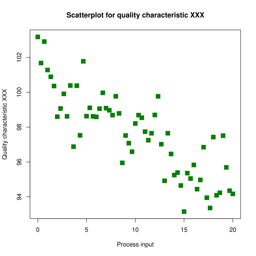
With a scatter plot, we get have clear view of all the data for two numerical variables.
2.3.1. Construction
This is a very simple process. A detailed explanation can be found here.
2.3.2. Interpretation
A scatter plot primarily helps us understand the relationship of the two variables. We can roughly infer the correlation and possibly the variability of the data.
2.4. Dot Plots
A dot plot can only visualize uni-variate data.
2.4.1. Interpretation
With a dot plot we can begin to identify more properties of a distribution, including:
- Central tendency
- Shape
- Spread
2.5. Stacked Dot Plots
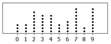
A dot plot with a twist. In this dot plot, we do not just plot data on a single horizontal line. Instead, with each next piece of data we stack the data points.
2.5.1. Interpretation
The higher the stack gets, the more data there is with that corresponding \(x\) axis value. We can easily infer the following:
- Central Tendency
- Skew
- Shape
- Spread
2.6. Histograms

It is the perfect alternative to a dot plot, when it comes to larger datasets. Instead of representing each observation with a dot, the histogram makes use of bins.
2.6.1. Interpretation
From a histogram, we can read the following:
- Data density
- Central Tendency
- Skew
- Shape
- Spread
- Outliers
When identifying outliers on a histogram, it is a guessing game.
2.7. Box Plots


The box part of the box plot contains 50% of the data. Inside the box there is a thick line, which is exactly at the median of the distribution. The outer lines of the box are the first and third quartile. The whiskers can extend up to \(1.5*IQR\) away from the quartiles, but not always.
\begin{array}{l} \text{max upper whisker reach} = Q3 + 1.5 * IQR \\ \text{max lower whisker reach} = Q1 - 1.5 * IQR \\ \end{array}Any outlier will always be past the maximum reach of each whisker.
2.7.1. Interpretation
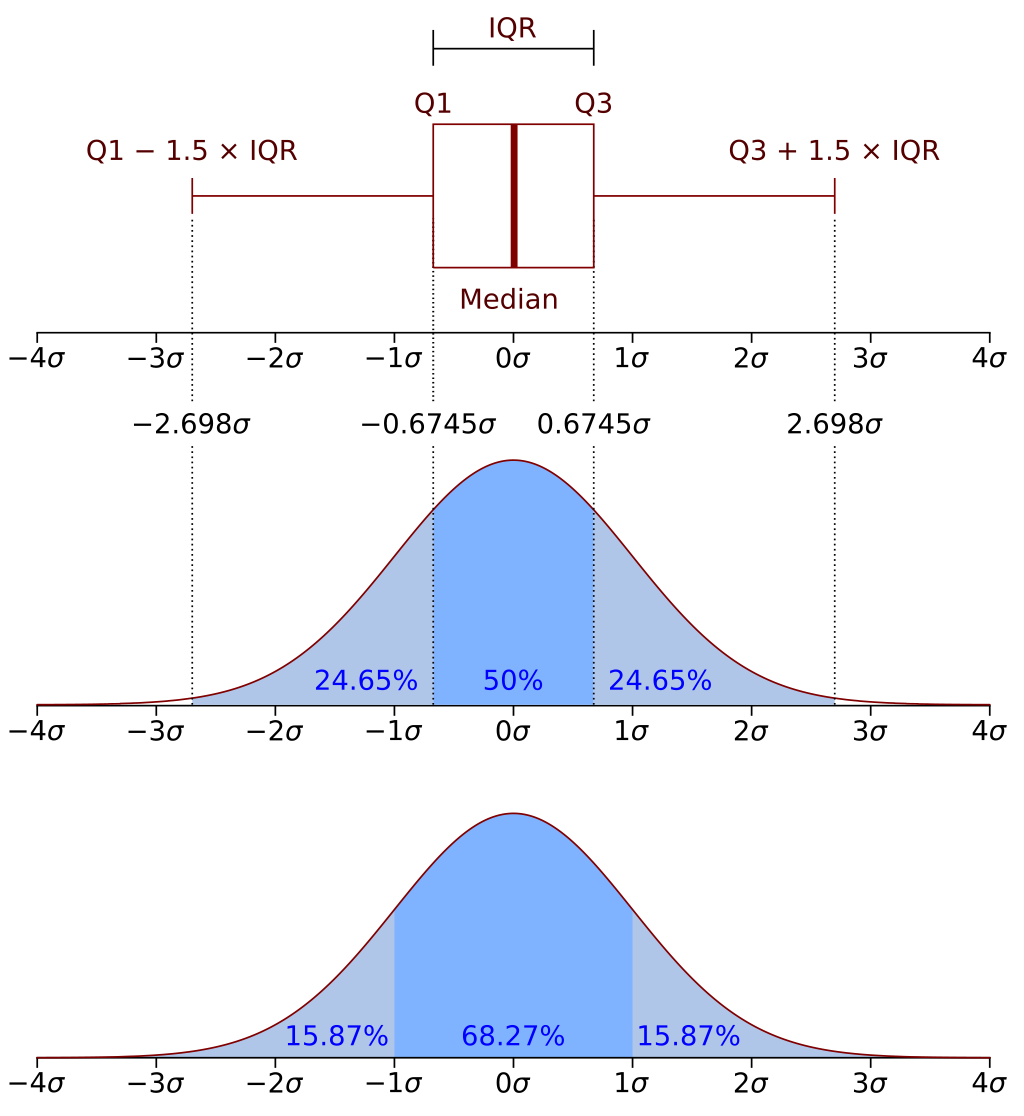
- The position of the median line relative to the edges of the box, tells us the skewness of the distribution.
3. Descriptive Statistics
3.1. Percentiles
A percentile exactly indicates the position of a value in a distribution. The location of a percentile can be computed with:
\[ \frac{P}{100} * (n+1) \]
3.2. Quartiles
A quartile also gives us an idea about the location of some value in the distribution. It divides our data into four equal parts. It allows us to easily understand larger datasets.
- Q1
- The first quartile is also the 25th percentile
- Q2
- The second quartile is also the 50th percentile
- Q3
- The third quartile is also the 75th percentile
3.2.1. Inter-quartile Range
Between Q3 and Q1, we can find 50% of the data. This range is also called the IQR, which can be later used to find outliers.
\[ IQR = Q3 - Q1 \]
3.3. Mean
With the mean, also called the average we can figure out the center of a data distribution. There are two kinds of means.
3.3.1. Sample Mean
Denoted by \(\bar{x}\), it is computed from \(n\) observations in a sample. It can be calculated by
\[ \bar{x} = \frac{x_1 + x_1 + \cdots + x_n}{n} \]
The primary characteristic of this mean is that it is only an estimate of the population mean.
3.3.2. Population Mean
Denoted by \(\mu\), represents the mean of the whole population. It is calculated the same way, except that it uses the entire population \(N\).
3.3.3. Usage of the Mean
A mean is a good representation fo the centrality of a distribution, as long as there are no outliers. Its value is highly susceptible to outliers and can be a very poor representation of the dataset. Despite this disadvantage it is still quite broadly used, because there are few populations with influential outliers.
3.4. Median
When calculating the median, the data is split in half. We can find the location of the median with \((\frac{n+1}{2})^{th}\). If the size of the data set is even, the median is the average of the two middle values.
The median is also the 50th percentile, and the second quartile.
3.5. Trimmed Means
Since the sample mean can at times be a bad representation of the distribution, we often resort to the median. To not lose the benefits of either, we can compute the trimmed mean. A trimmed mean is calculated by eliminating the smallest and largest \(n%\) of the samples.
- A 5% to 25% trimmed mean will give us the perfect range.
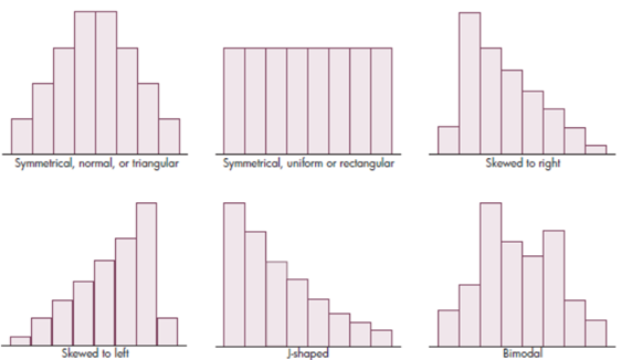
3.6. Skew
When a distribution looks to have a longer tail on one side rather than the other, it is said to have a certain skew. There are two ways a distribution can be skewed.
- Right/Positive Skew
- When a distribution has a long right tail.
- Left/Negative Skew
- When a distribution has a long left tail.
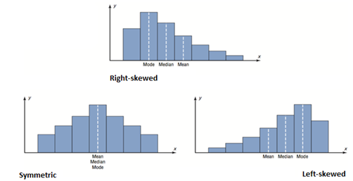
We can also identify the skew of a distribution by looking at its mean and median. The mean will be closer to the tail.
- Right Skew
- mean < median
- Left Skew
- mean > median
3.6.1. Treating Extremely Skewed Data
If we have a dataset with in which that data is extremely skewed, we can use a log transformation for easier modeling. With a transformation, the outliers will become much less prominent. The downside of using log transformation is that it is more difficult to interpret.
3.7. Distribution Shape
There are 4 main properties when it comes to distribution shapes.
- Uni-modal
- Single prominent peak
- Bimodal
- Two prominent peaks
- Multimodal
- Multiple prominent peaks
- Uniform
- No apparent peaks
The prominent peak of a distribution can also be called the mode. It is the value with the most procurances in a dataset.
3.8. Frequency
The frequency in statistics is equal to the number of times certain variable occurs in a dataset.
3.8.1. Relative frequency
It is the proportion of that value in a dataset.
\[ f = \frac{\text{number of times the value occurs}}{\text{number of observations in dataset}} \]
The sum of all relative frequencies should add up to 1.
- Frequency Distribution
- A table of frequencies and relative frequencies.
3.9. Sample Variance
This statistics describes the variability of a dataset. We start by comparing all the observations to the mean (this is called the deviation), we then square all these distances (to get a positive value) and take an average. The result of this calculation is the sample variance.
\[ s^2 = \frac{\sum_{i=1}^n {(x_i - \bar{x})^2}}{n - 1} \]
There is an alternate way to express this:
\[ s_xx = \sum(x_1 - \bar{x})^2 = \sum x_i^2 - \frac{(\sum x_i)^2}{n} \]
The proof of this is in 5.
3.10. Sample Standard Deviation
Just like the sample variance, this statistics describes the variability of a distribution.
\[ s = \sqrt{s^2} \]
What makes the standard deviation special, is that *all the data is within 3 standard deviations relative to the mean.
3.11. Population Variance
It is roughly the average squared deviation from the population mean, denoted by \(\sigma^2\). The differentiating factor from the Sample Variance is that *it uses the entire population \(N\).
\[ \sigma^2 = \frac{\sum_{i=1}^n {(x_i - \bar{\mu})^2}}{n - 1} \]
3.12. Population Standard Deviation
Just like the Sample Standard Deviation, it is the square root of the population variance.
\[ \sigma = \sqrt{\sigma^2} \]
All other properties remain the same.
3.13. The Range
The range, primarily measures the spread of a distribution, but it can also be interpreted as the simplest measure of variation.
\[ \text{Range} = X_{max} - X_{min} \]
- Disadvantage
- It only considers the two most extreme observations.
3.14. Outliers
As stated before, outliers are pieces of data which our outside the range of the \(Q1/Q3 \pm 1.5*IQR\) scope.
- Importance of outliers
- Identifying extreme skew
- Identifying collection/entry errors
- Providing insight into data features
3.15. Statistical Robustness
- If we have a skewed distribution, it is better to use the median and IQR to describe the center and spread.
- However, for a symmetric distribution it is more helpful to use the mean and standard deviation. Here we use the mean because in symmetric distributions \(\text{median} \approx \text{mean}\).
3.16. Chebychev's Theorem
For any population. The percentage of data within the interval \(\mu \pm k\sigma\) is at least \(100(1 - \frac{1}{k^2})\) percent.
3.17. Empirical Rules
The empirical rule heavily relies on the Chebychev's Theorem, for measuring percentages of a distribution. For any symmetric distribution, we can apply the following rules:
- 68% of the data falls under \(\mu \pm 1 \sigma\)
- 95% of the data falls under \(\mu \pm 2 \sigma\)
- 99.7% of the data falls under \(\mu \pm 3 \sigma\)
3.18. Z Score
Z-scores are one of the most popular metrics for comparing a certain data point to the rest of the distribution. There are two types of z-scores, a population z-score and a sample z-score. The only difference is that they use the population and sample mean respectively, same applies for the standard deviations.
\[ z = \frac{x - \bar{x}/\mu}{s/\sigma} \]
3.19. Correlation
Correlation is a measure of how associated two variables are. The most commonly used type of correlation is the Pearson Correlation.
When thinking about correlation and association, we must remember that association does not imply causation.
3.19.1. Covariance
With covariance, we can measure in which direction the linear relationship of two variables is.
\[ cov(x,y) = s_{xy} = \frac{\sum_{i=1}^n (x_i - \bar{x})(y_i - \bar{y})}{n-1} \]
- $cov(x,y) > 0
- \(x\) and \(y\) tend to move in the same direction
- $cov(x,y) < 0
- \(x\) and \(y\) tend to move in the opposite direction
- $cov(x,y) = 0
- \(x\) and \(y\) are independent
3.19.2. Correlation Coefficient
In order to measure, correlation, we need some numerical value. The correlation coefficient tells us two things about the relationship: the strength and direction of correlation between two variables.
- It can range between -1 and 1
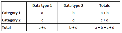
3.20. Sample Proportions
With categorical data, it is useful to construct a tabular frequency distribution. The general formula for a sample proportion is as follows:
\[ p = {x \over n} \]
Given categorical data and their frequencies we can construct a contingency table.
3.21. Hypothesis Testing
When testing a hypothesis, we need two. One being the null hypothesis (\(H_0\)) and the other, alternative hypothesis (\(H_a\)).
- Null Hypothesis
- There is nothing going on
- Alternate Hypothesis
- There is something going on.
When testing a hypothesis, we make a discussion as to how unlikely the unlikely outcome is. The entire process of testing a hypothesis is based on the assumption that the null hypothesis is true.
4. Probability
4.1. Sample Space
The way we denote the sample space of an experiment is by \(S\). This is the set of all possible outcomes of that experiment.
4.2. Events
An event is a set which contains certain outcomes contained the sample space \(S\). If an event only has one outcome, it is called simple, otherwise we call it compound. If the outcome of an experiment is contained in the event \(A\), we can say that the event \(A\) has occurred.
4.3. Axioms of Probability
When conducting an experiment, we use probability to precisely measure the change that some event \(A\) will occur. All probability should satisfy the following axioms.
- For any event \(A\), \(P(A) \ge 0\)
- \(P(S) = 1\)
- If \(A_1, A_2 A_4, \dots\) is an infinite collection of disjoint events, then \(P(A_1 \cup A_2 \cup A_3 \cup \cdots) = \sum_{i=1}^\infty P(A_1)\)
4.4. Properties of Probability
- \(P(A) + P(A^\prime) = 1\)
- \(P(A) \le 1\)
4.5. Operations with Probability
4.5.1. Union
If we have events that are not mutually exclusive, if we add the probabilities, we double-count their intersection, thus it must be subtracted.
\[ P(A \cup B) = P(A) + P(B) - P(A \cap B) \]
When it comes to the union of 3 events:
\[ P(A \cup B \cup C) = P(A) + P(B) + P(C) - P(A \cap B) - P(A \cap C) - P(B \cap C) + P(A \cap B \cap C) \]
It is important to notice that the last probability is added and not subtracted.
4.6. Systematic Approach to Solving Probabilities
quite a mouth-full
If we have some compound event \(A\), which consists of \(n\) events \(E_i\), we can solve for \(P(A)\) using the following rule.
\[ P(A) = \sum_{E_i \in A} P(E_i) \]
If we can find a way to define all events \(E\), we can solve for \(P(A)\) in terms of some constant.
4.7. Uniform Probabilities
If we have some sort of experiment in which the outcome of some event is equally as likely as that of another, we say that we have equally likely outcomes. This means that for each event, the probability is \(p = {1 \over N}\) where \(N\) is the number of events. The simplest example of this is a coin toss or a die roll.
4.8. Product Rule for Ordered Pairs
If we have an event which consists of ordered pairs of objects and we want to know the number of pair there are, we can use the below mention proposition. What we mean by an ordered pair, is a set of two elements, where the order of the elements matters.
If the first element of an ordered pair can be selected in \(n\) ways, and for each of these \(n\) ways the second element of the pair can be selected in \(m\) ways, then the number of pair is \(n*m\).
It can be very useful to build something called a tree diagram. With this diagram, we can visualize all possibilities.
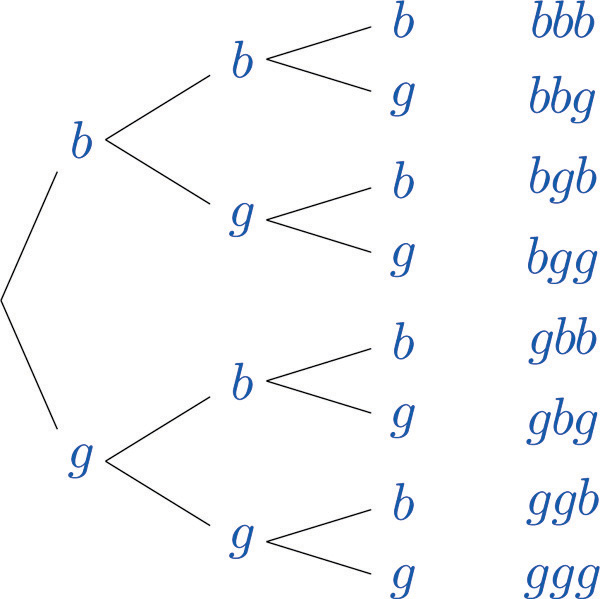
When looking at the graph from left to right, each line connecting two nodes, is called an n-th generation branch. With each new branch, \(n\) increases.
With the tree diagram, we can easily calculate givens and conjunctions.

4.9. Permutations
A permutation is an ordered combination. Just like in combinations, we either can or cannot repeat elements.
4.9.1. Permutations with Repetition
If we are trying to select from \(n\) objects, but that number \(n\) dose not decrease each time we select an item (the set is not exhaustive), we can model the number of permutations with:
\[ n^r \]
Where \(r\) is the number of times we are choosing from \(n\).
4.9.2. Permutations without Repetition
Each time we select an element from \(n\) objects, the next time we do so again, we have \(n-1\) objects. The simplest way to express this is by using a factorial (n!). A single factorial, however does not let us represent a specific number of ways we want to permute. Since the factorial relies on multiplication, we just need to divide by the remaining permutations. This gets us the following formula:
\[ P(n,r) = {n! \over (n-r)!} \]
4.10. Combinations
A combination is a subset, that has no order. For this subset, we can consider two states where we can repeat elements or cannot repeat elements.
4.10.1. Combinations without Repetition
It is a permutation without repetition and without order. The formula is very similar, the only difference is that we need to account for all the values which were ordered but now do not matter. We do this by dividing by \(r!\).
\[ C(n,r) = {n! \over { r!(n-r)! }} \]
Another way to go about this is to use Pascals Triangle, this is out of scope.
4.11. Conditional Probability
The probability of an event might not always be straight-forward, and we may need to find ways to figure it out. With conditional probability, we can find how some event \(A\) might affect \(B\). We use the notation \(P(A\vert B)\) to represent probability of A given that B has occured. The definition of conditional probability for two events is:
\[ P(A\vert B) = \frac{P(A \cap B)}{P(B)} \]
- Multiplication rule for \(P(A \cap B)\)
- This rule is very important for solving certain problems where we know \(P(A\vert B)\) and \(P(B)\). With these two and the above formula for conditional probability, we can know that \(P(A\cap B) = P(A\vert B)* P(B)\).
4.12. Bayes' Theorem
This theorem allows us to compute the probability of some event, based on knowing other conditional probabilities concerning that event. In this theorem, it is assumed that two events \(A\) and \(B\) are independent. The formula is as follows:
\[ P(A\vert B) = \frac{P(B\vert A) * P(A)}{P(B)} \]
You can further expand this formula using the Law of Total Probability.
\[ P(A\vert B) = \frac{P(B\vert A) * P(A)}{P(B\vert A) * P(A) + P(B \vert \neg A) * P(\neg A)} \]
4.13. Independence
In a lot of previous concepts, we have assumed independence. Independence occurs, if
\[ P(A \vert B) = P(A) \]
Another way we can check for independence is with the multiplication rule. Which states that
\[ P(A \cap B) = P(A) * P(B) \]
We can also use this the other way around, if we know that two events are independent, we can find the probability of their conjunction by multiplication. This concept can be extended to any number of events.
5. Appendix 1
\[ \bar{x} = \frac{\sum{x_i}}{n} \]
\[ \bar{x}^2 = \frac{\sum{x_i}^2}{n^2} \]
\[ \sum{(x_i - \bar{x})^2} = \sum{(x_i - \bar{x})(x_i -\bar{x})} = \sum{x_i^2 -2x_i\bar{x} + \bar{x}^2} \]
We apply the distributive identity to the second expression: \(\sum{C * f} = C * \sum{f}\) where \(C\) would be \(2\bar{x}\).
As per the first definition above \(\bar{x} = \frac{\sum{x_i}}{n}\), therefore \(\sum{x_i} = \bar{x}n\).
\[ = \sum{x_i^2} - 2\bar{x}(\bar{x}n) +\sum{\bar{x}^2} \]
Because \(\bar{x}\) is a constant, \(\sum{\bar{x}^2} = n\bar{x}^2\). This is according to \(\sum{c} = nc\).
\[ = \sum{x_i^2} - 2\bar{x}^2n + \bar{x}^2n = \sum{x_i^2} - \bar{x}^2n \]
\[ = \sum{x_i^2} - \frac{\sum{x_i}^2}{n^2} * n = \sum{x_i^2} - \frac{\sum{x_i}^2}{n} \]